Sensitivity analysis using Delta method #

Since our new feasible region is smaller, we are getting a sub optimal result (because we are minimizing).

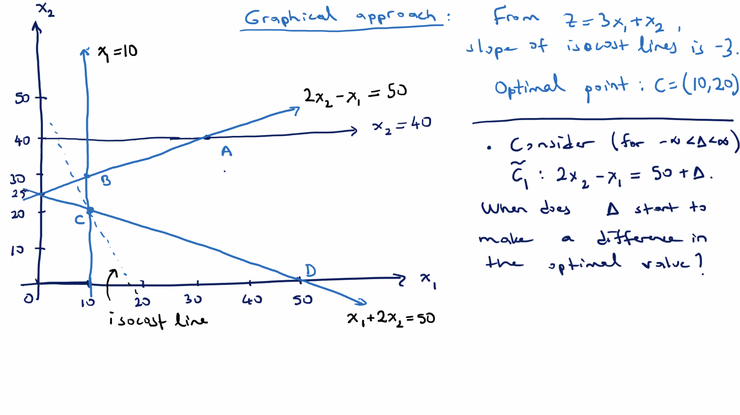
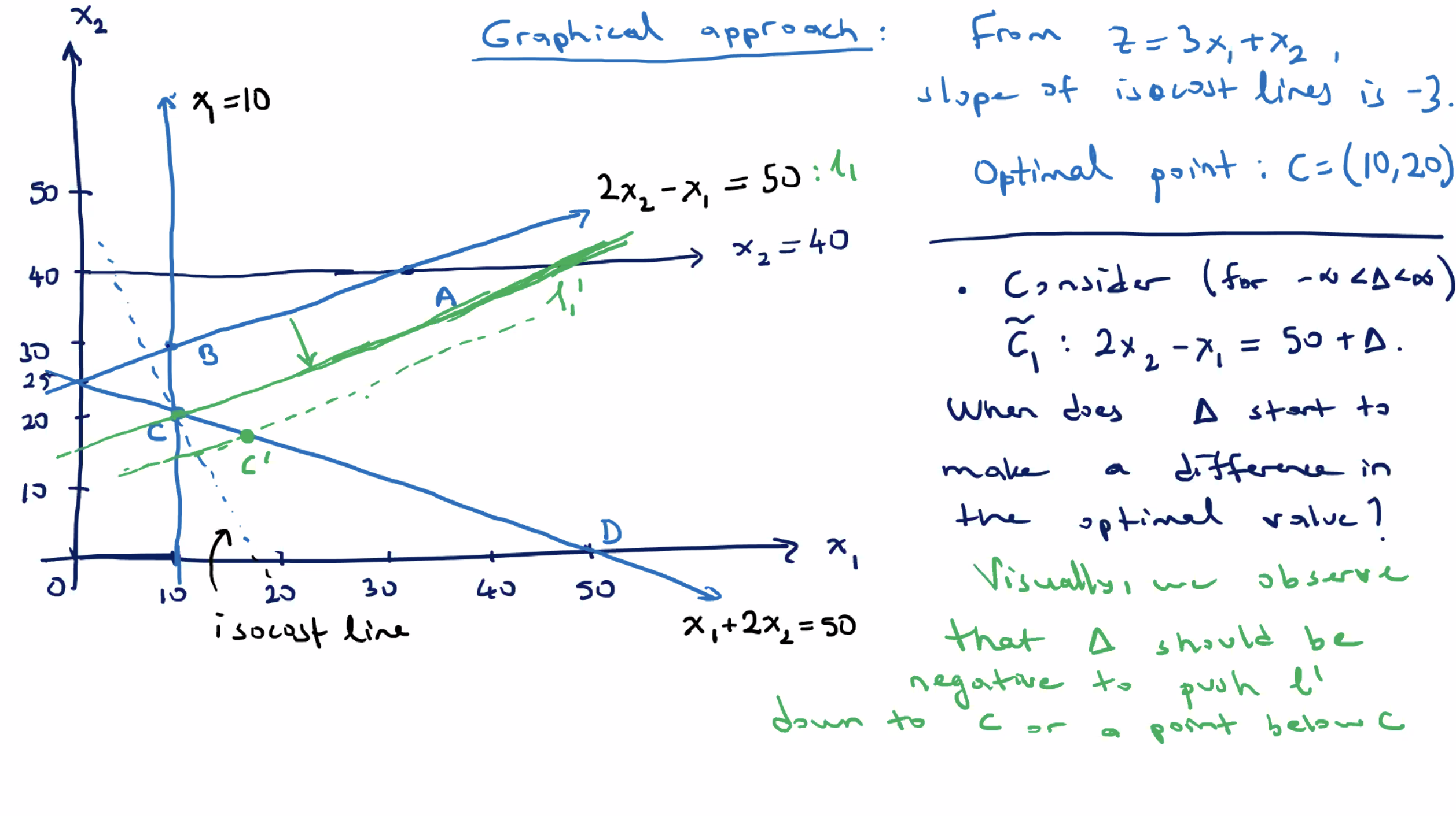
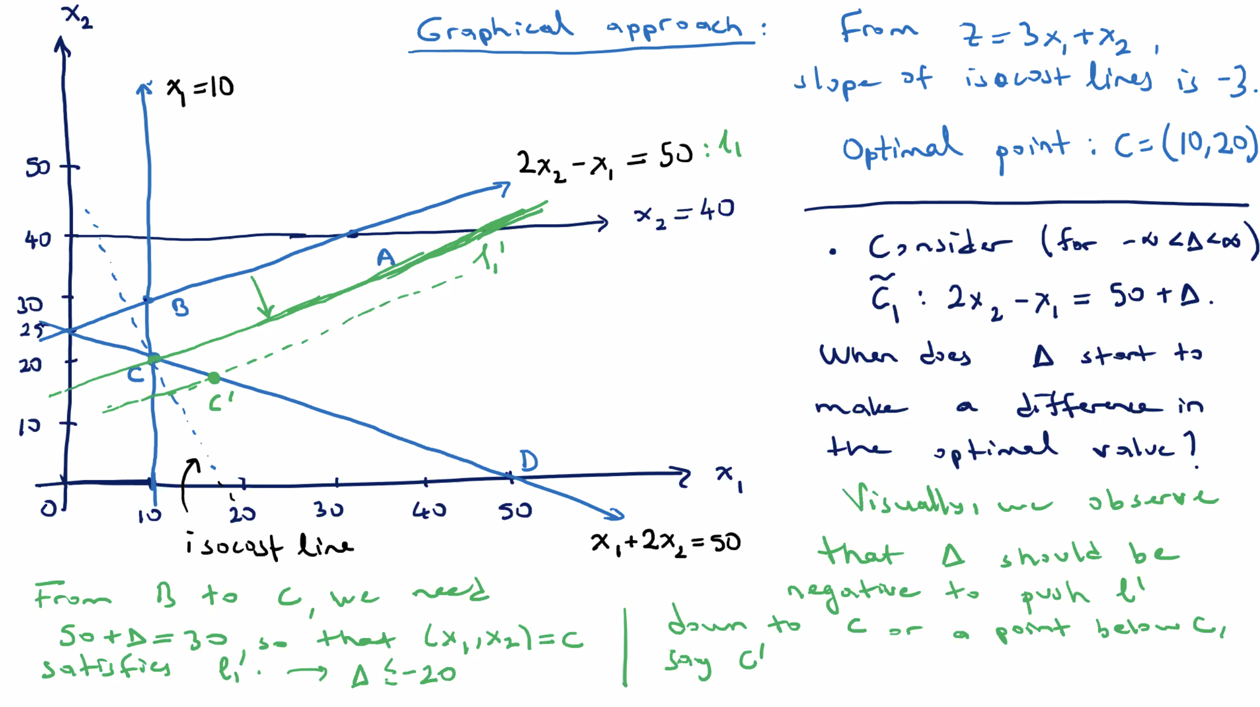
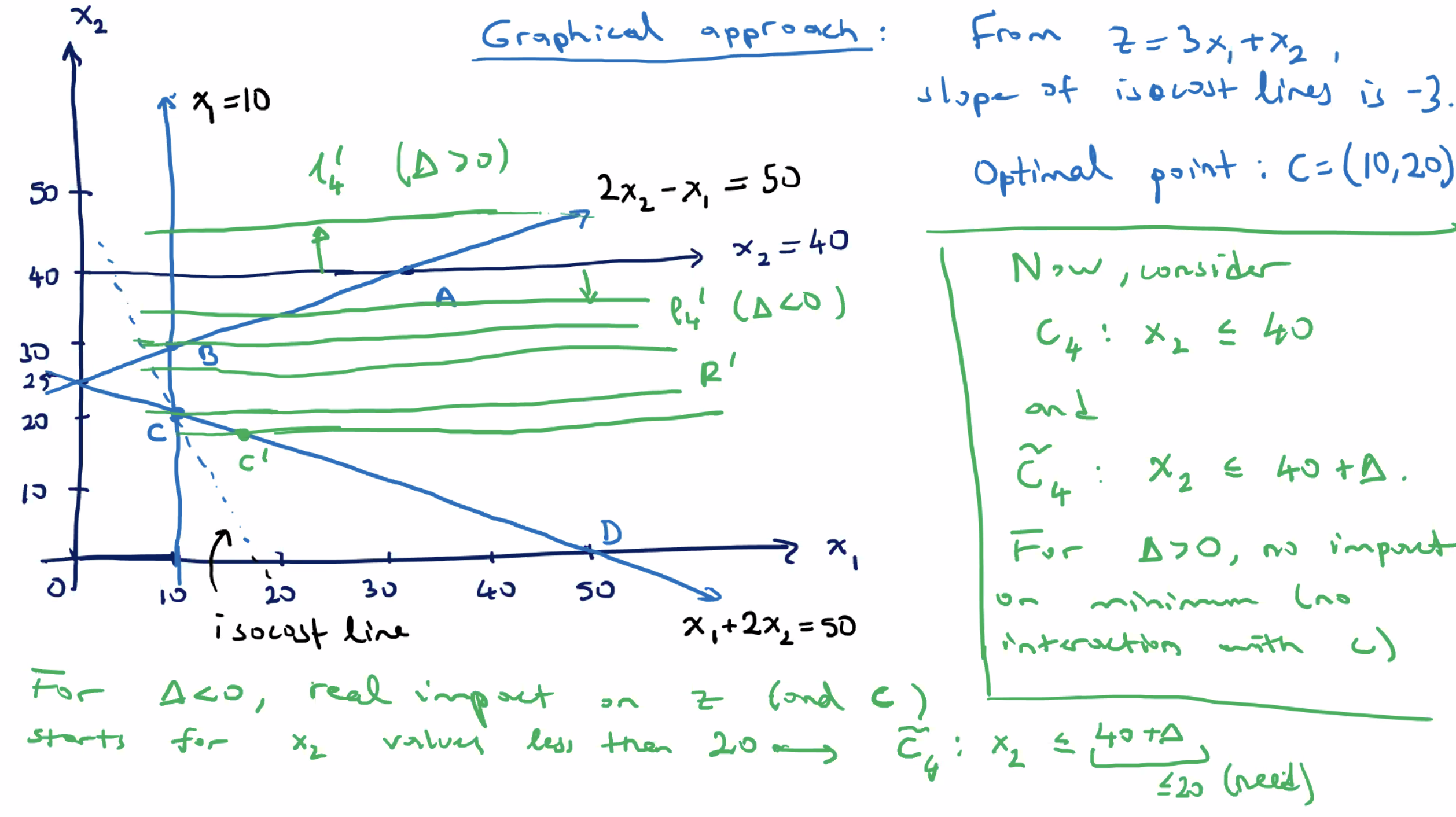
For this impact of \( \tilde{c_4} \) on \( z \) , we need \( \Delta \leq -20 \) .

• At \( \Delta = -20 \) , \( C=(10,20) \) is still the optimal solution.
• After that, for \( \Delta < -20 \) , it creates a new corner point \( C' \) .

For example, when \( \Delta=-21 \) , \( C' \) is the point with \( c_4' : x_2 \leq 40 - 21 = 19 \) and \( x_1 \) satisifies \( \ell_2 : x_1 + 2x_2 = 50 \) , so \( x_1 = 12 \) .

• the new point is \( C' = (12,19) \)
• new corresponding \( z \) value of \( z' = 55 \)

Since this is larger than the original \( z \) , it is a sub optimal solution (recall we are minimizing).

So can we identify this without graphing?

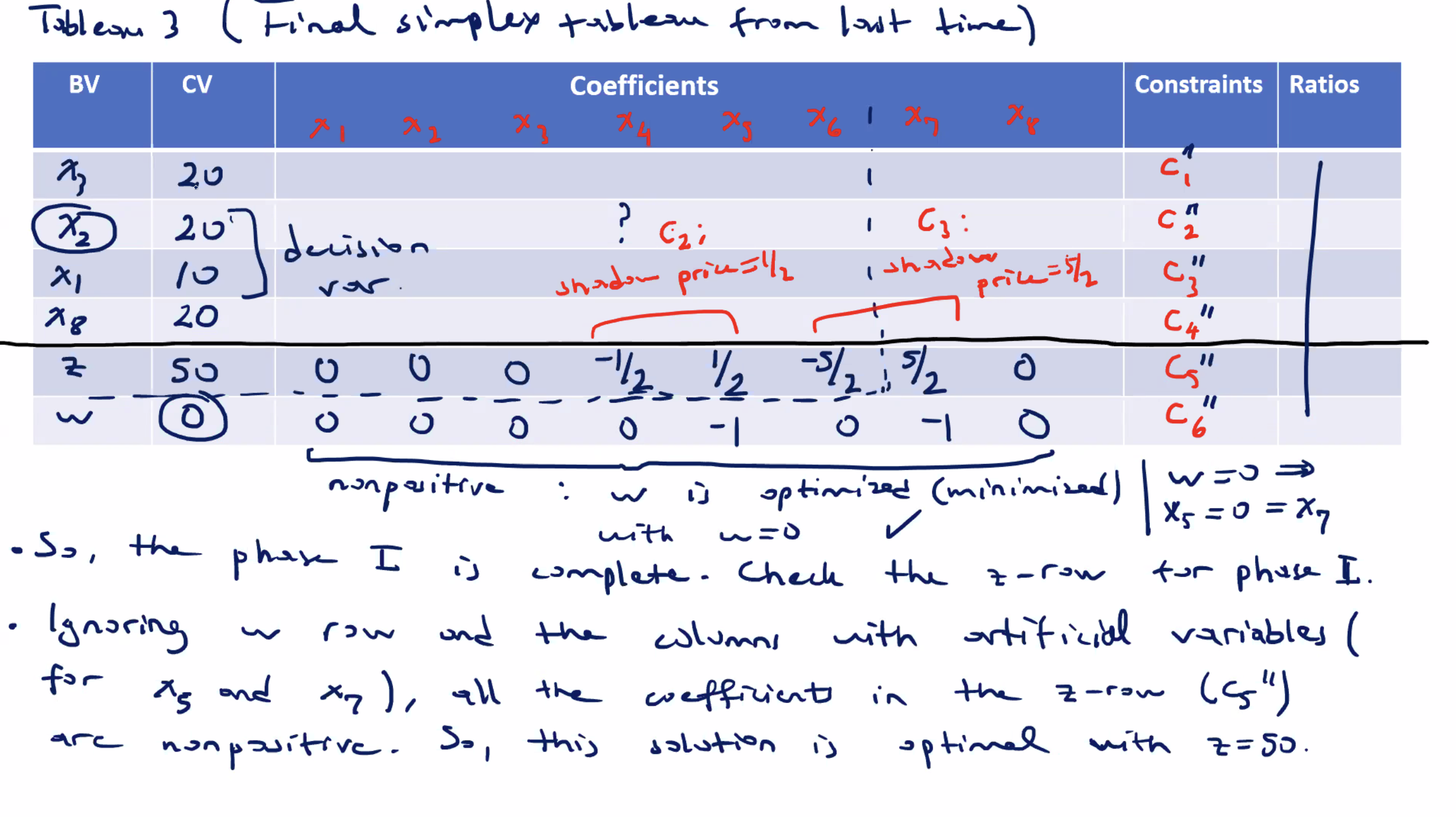
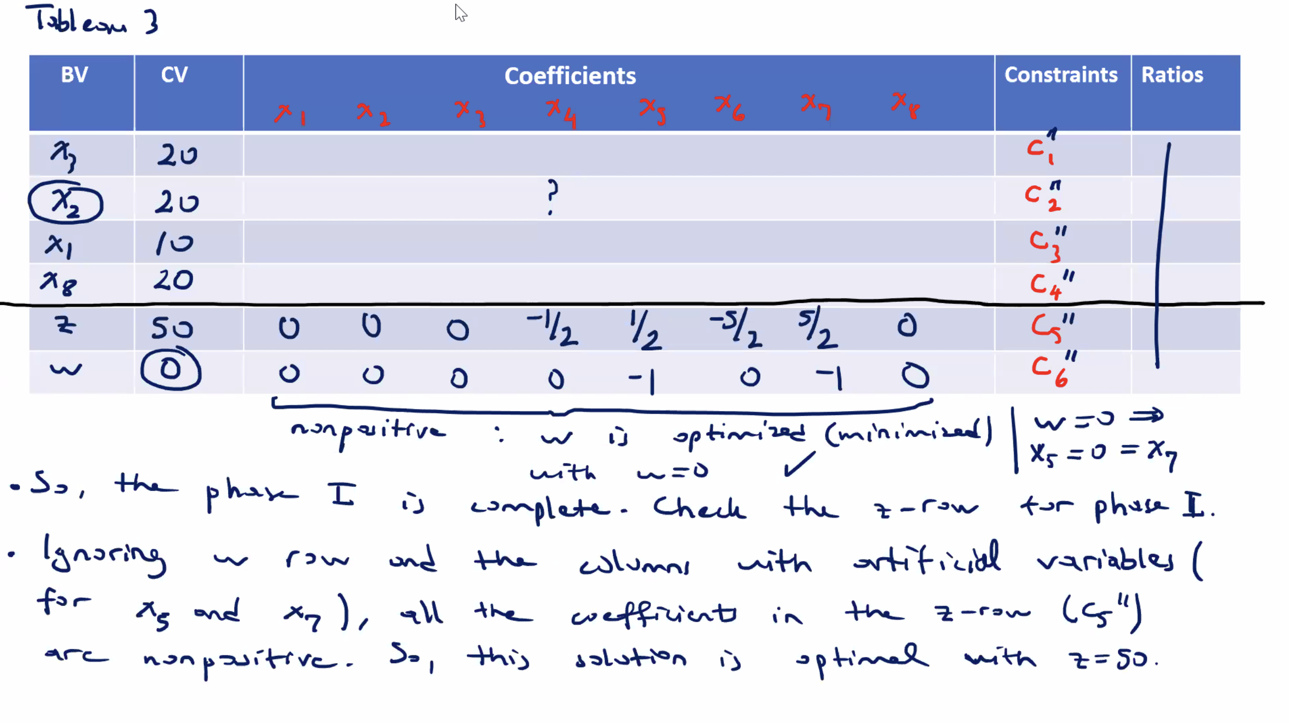
From the simplex tableau:

• check the current value column for the decision variables to see how big \( \Delta \) can be
  • observe that \( x_3 = 20 \) and \( x_8 = 20\) are the values for the slack variables of \( c_1 \) and \( c_4 \) respectively.
  • they are basic variables in the optimal BFS, so they have zero coefficient in the \( z \) -equation (last row) in the simplex tableau (which is why their shadow prices are 0)
  • However, from their values of \( x_3=x_8=20 \) , we can conclude that \( \Delta \) changes in their constraints impact the optimal solution when \( \Delta \) amount is at least \( 20 \) units (in the negative direction for this minimzation problem)

Look at the impact of changes in the coefficients of the decision variables on the optimal solution.

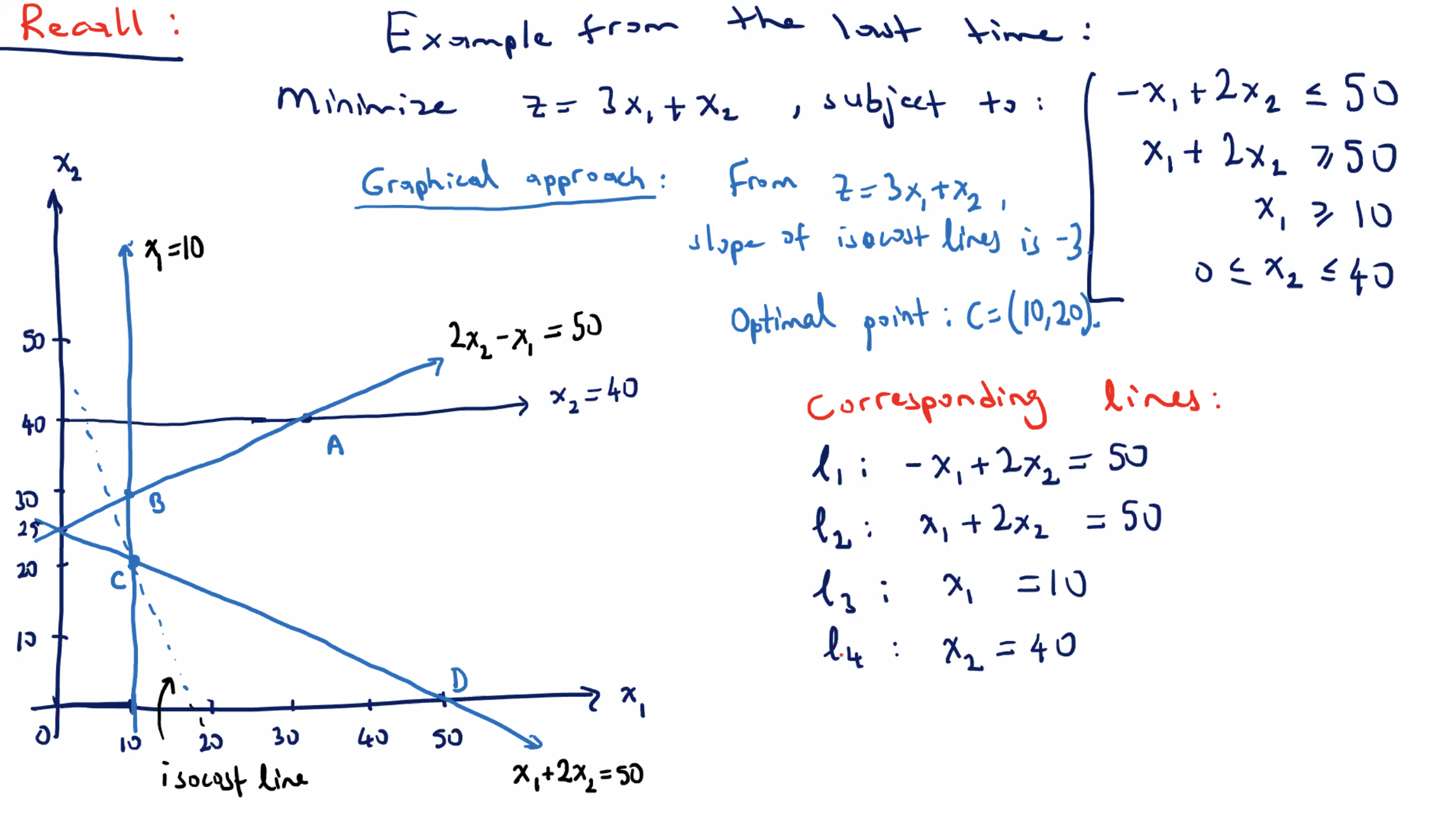
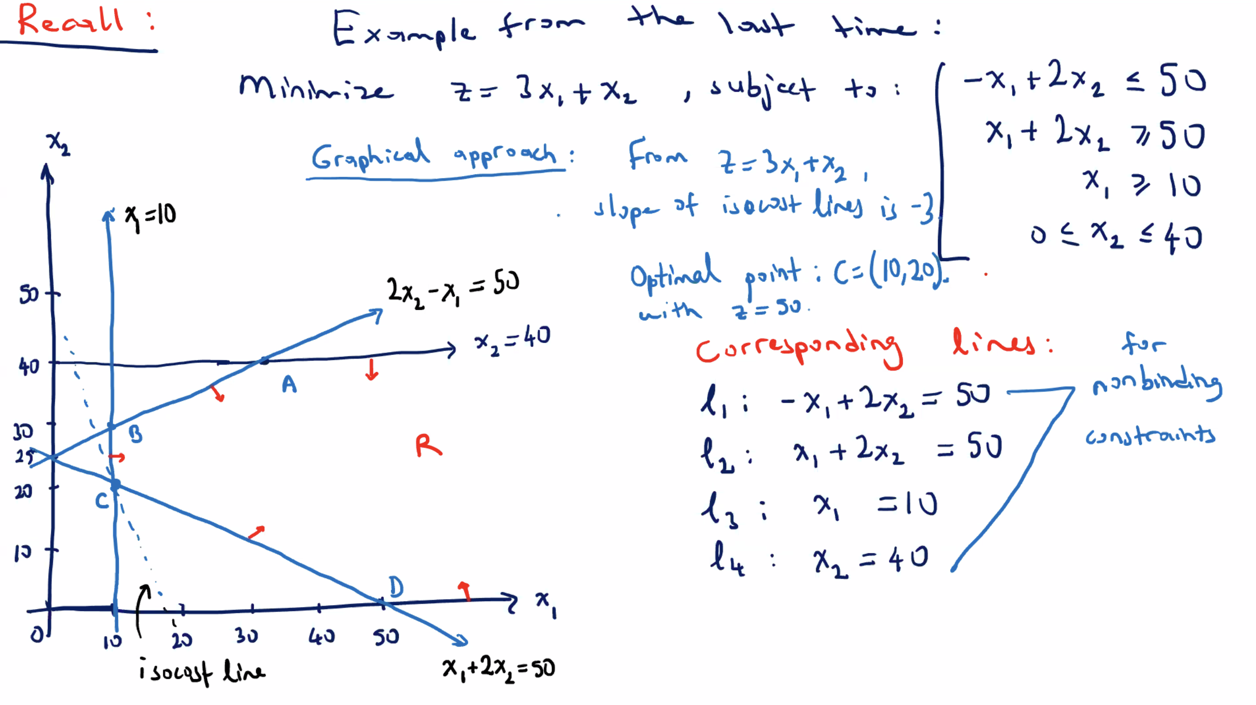
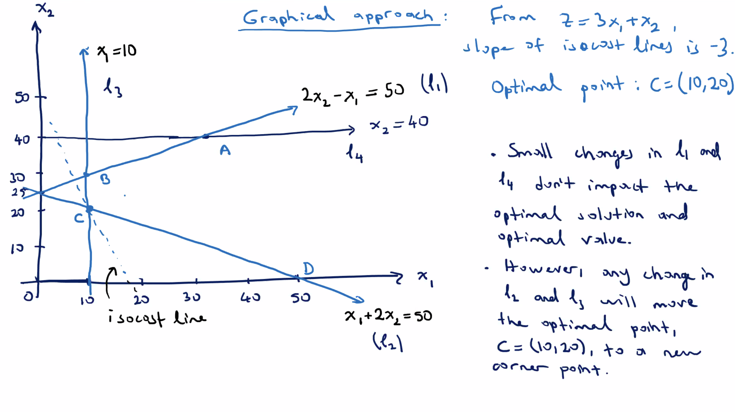
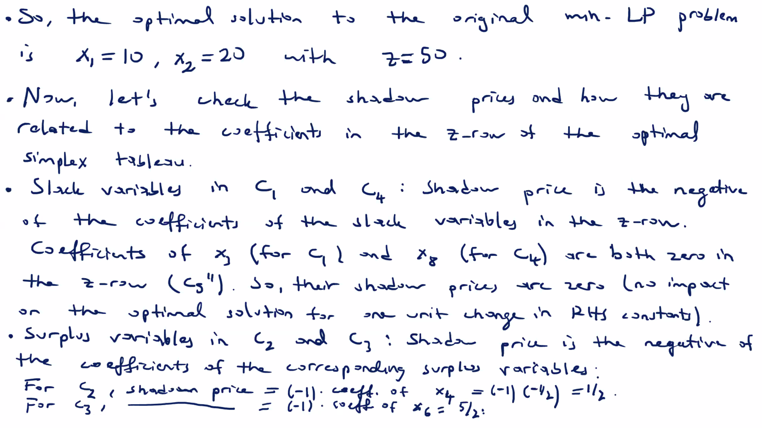
• Consider the same objective function, \( z= 3x_1 + x_2 \) .
• What happens if it is changed to \( z = 4x_1 + x_2 \) ?
• The isocost lines will have the slope \( -4 \) . We can check graphically that it doesn’t change the optimal solution with the same constraints, in this example
• Similarly, we can check that an increase in the coefficient of \( x_2 \) will not impact the solution