Graph basics #

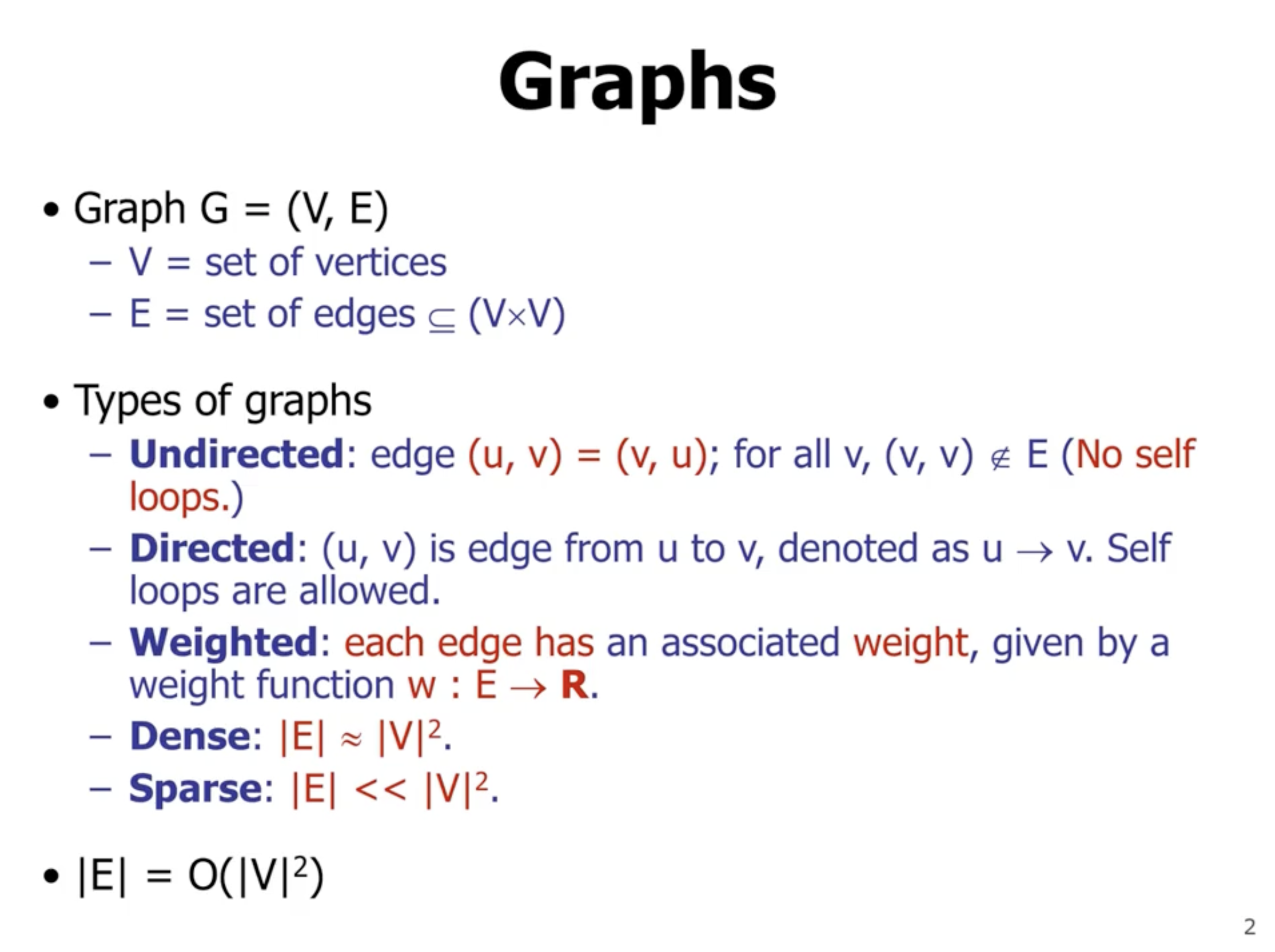
In basic graphs, self loops and multiple edges between vertices are not considered. The number of edges are calculated by

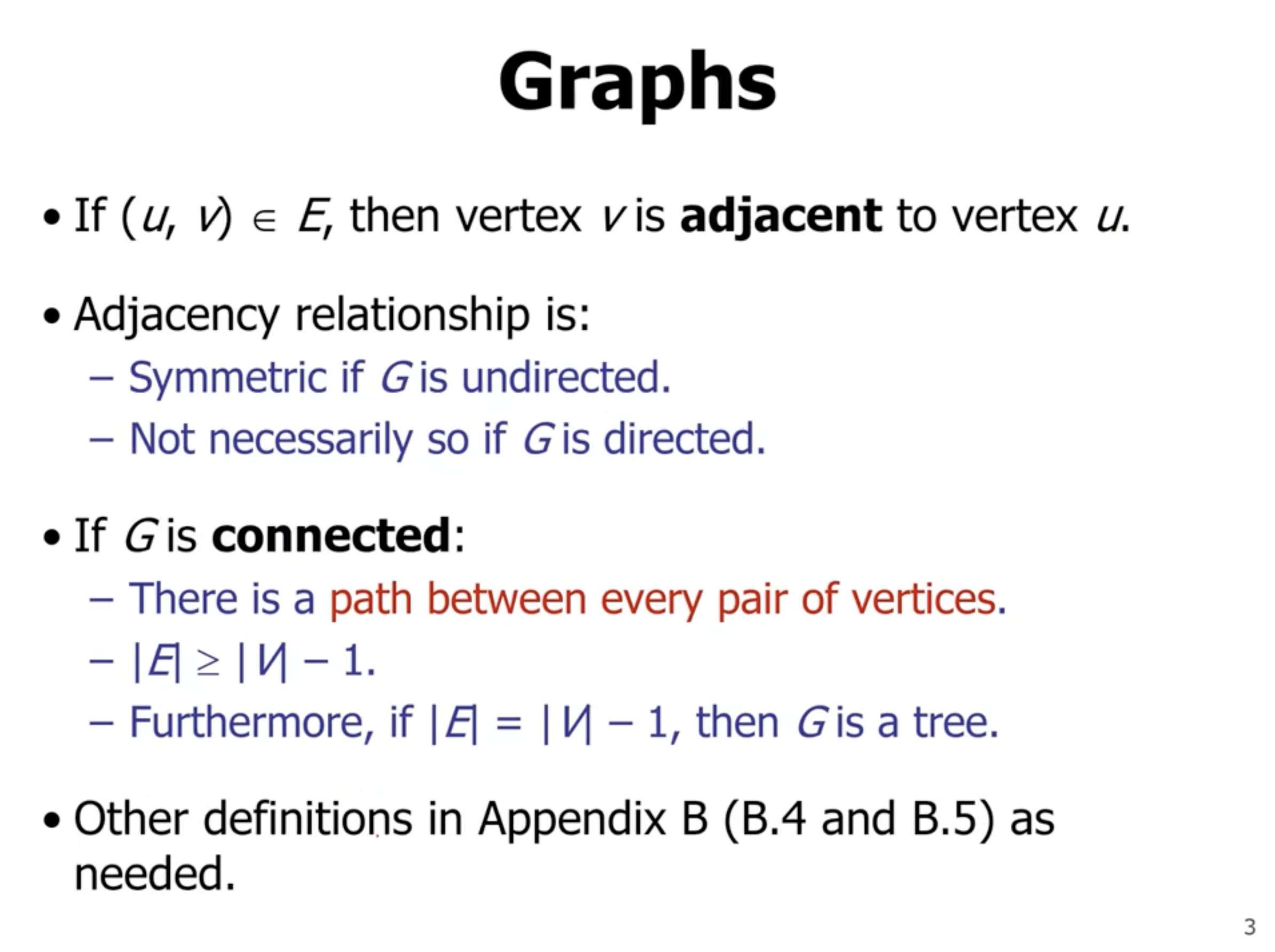
A directed graph is

• strongly connected if there is a path from any vertex to any other vertex in the direction of edges
• unilaterally connected if for any 2 vertices there is a directed path to and from each vertices
• weakly connected if there is a path from any vertex to any other vertex, but not in the direction of edges

Representing graphs #

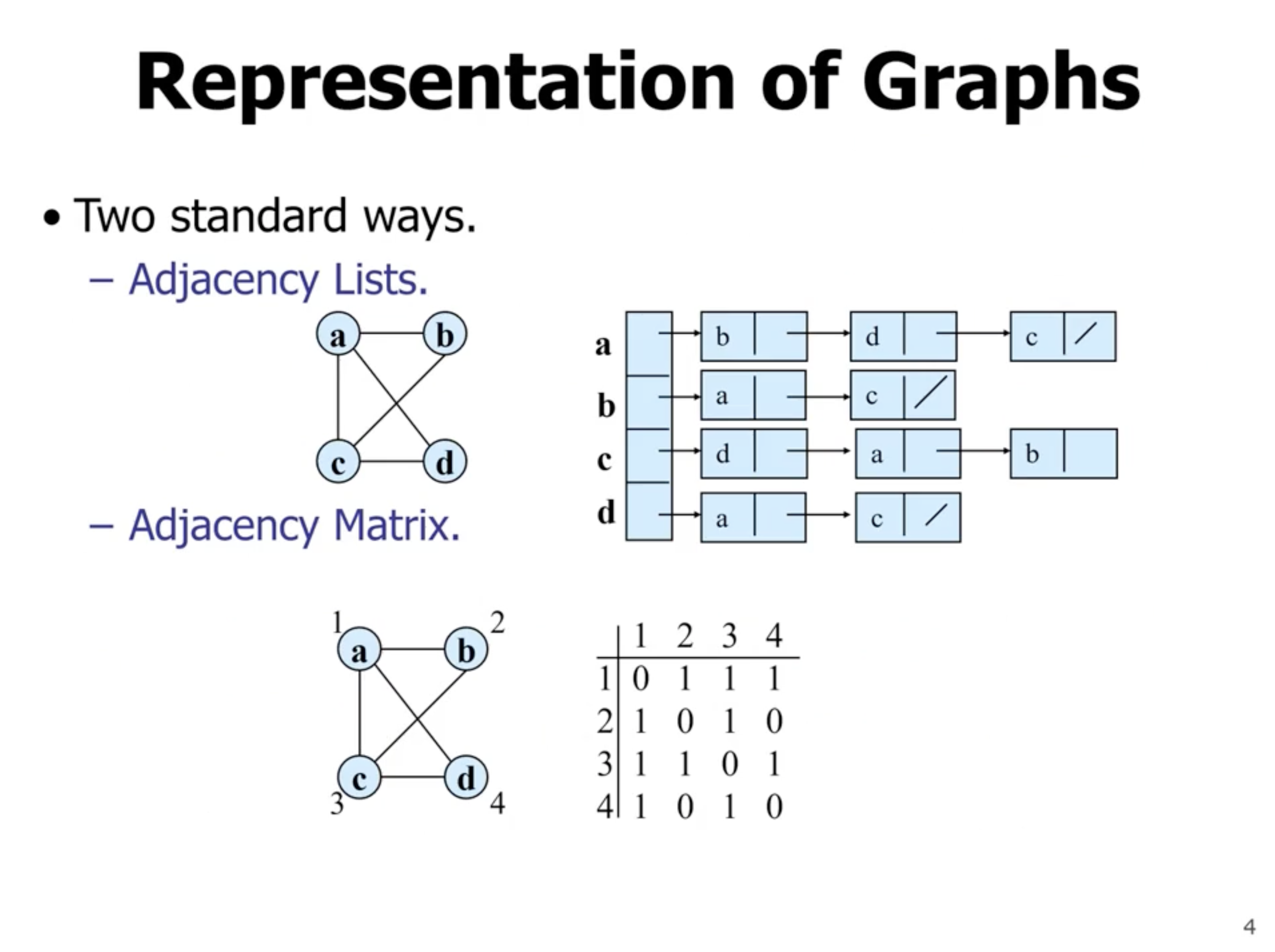
Adjacency lists #

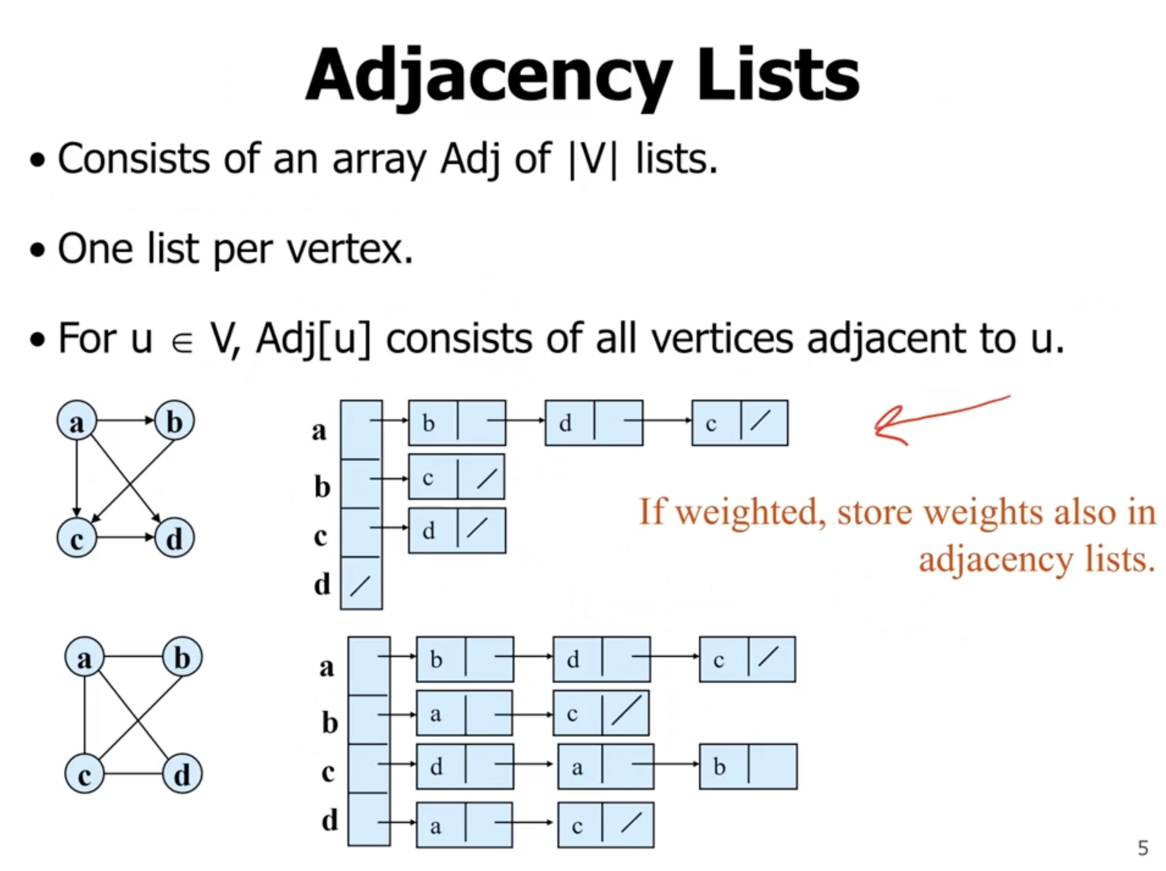
Note: The total length of linked lists for directed graph is less than the total length of linked lists for the undirected graph in this example.

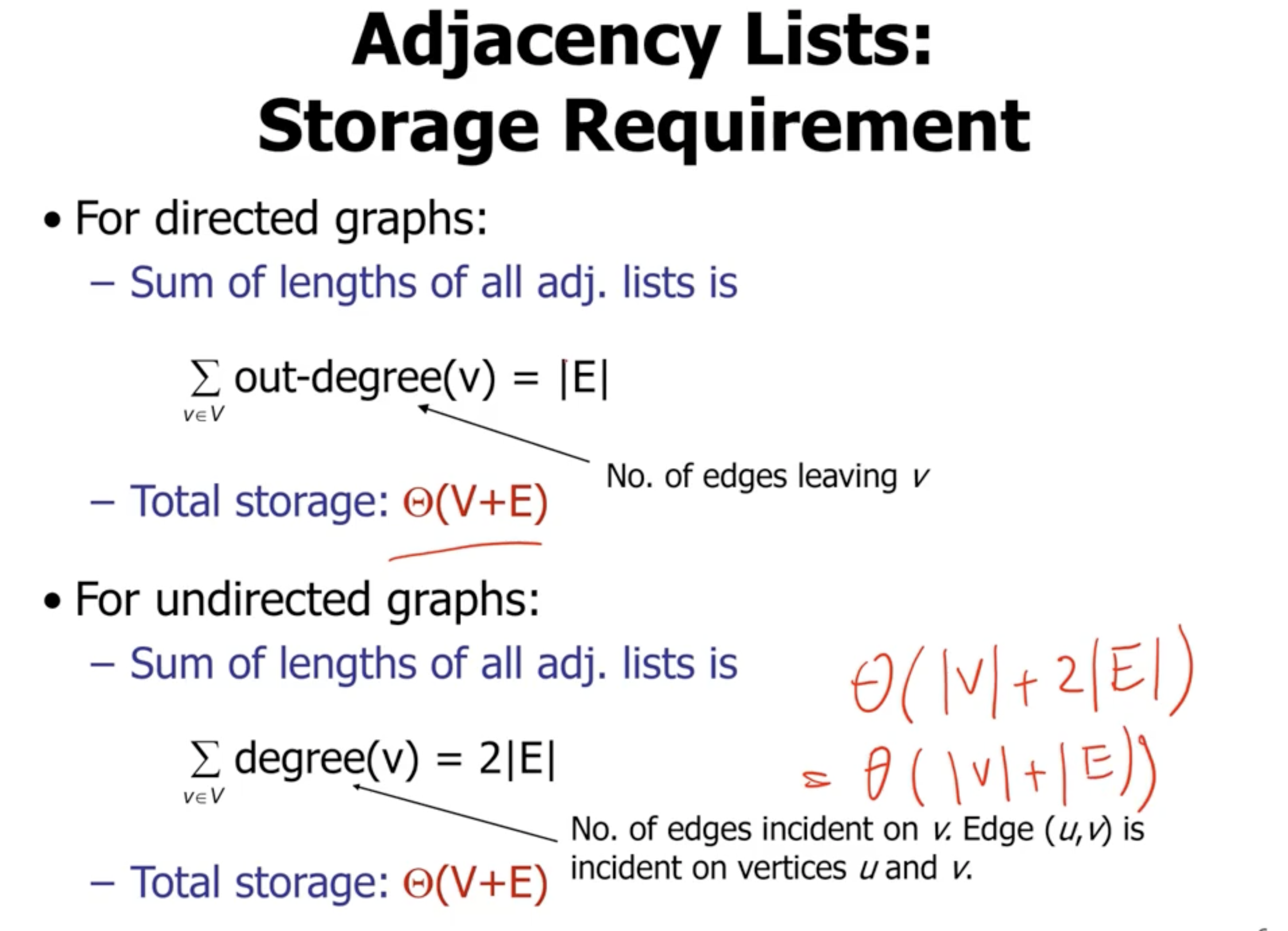
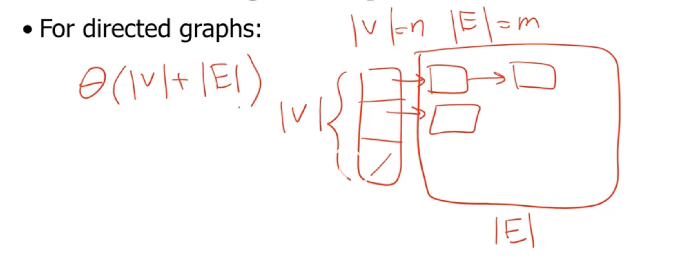
The degree of a vertex \( u \) is the number of edges connected to \( u \) . In a directed graph: the out-degree is the number of edges leaving, and the in-degree is the number of edges arriving.

Adjacency matrix #

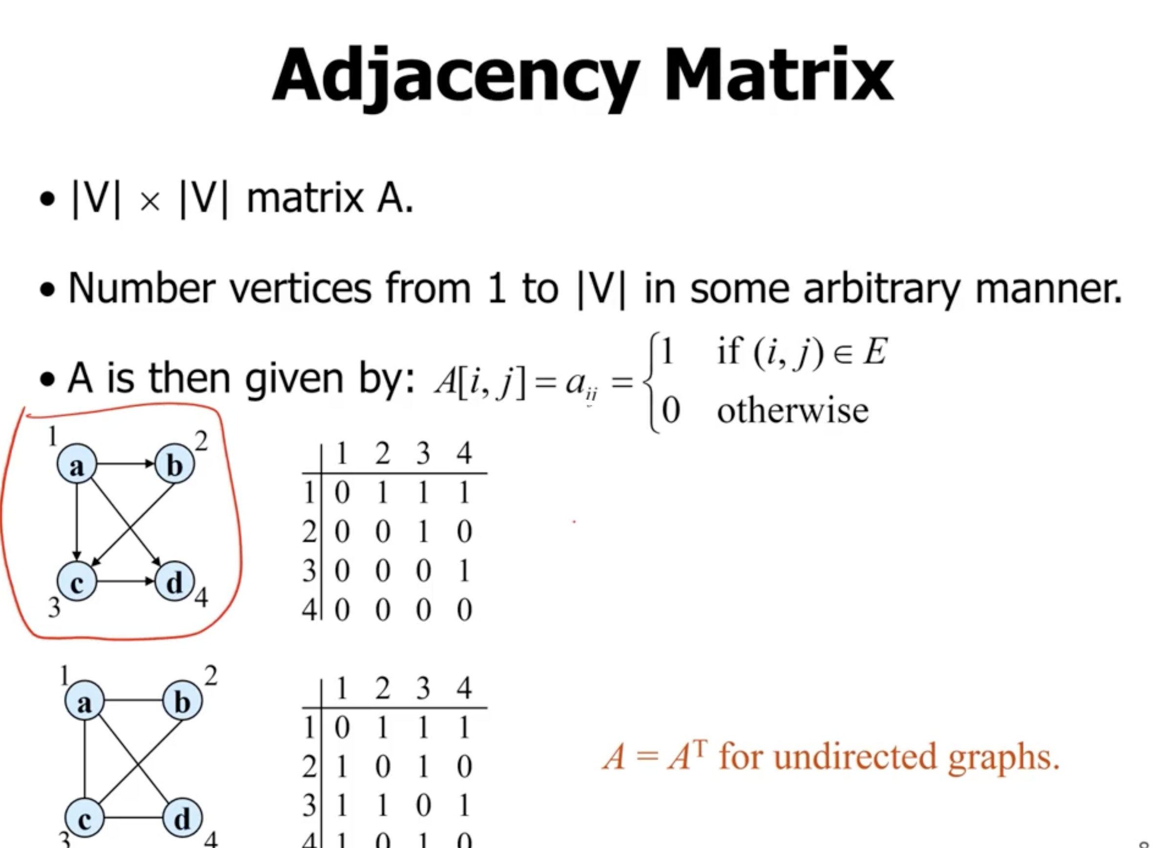
In an undirected graph, the adjacency matrix is symmetric.

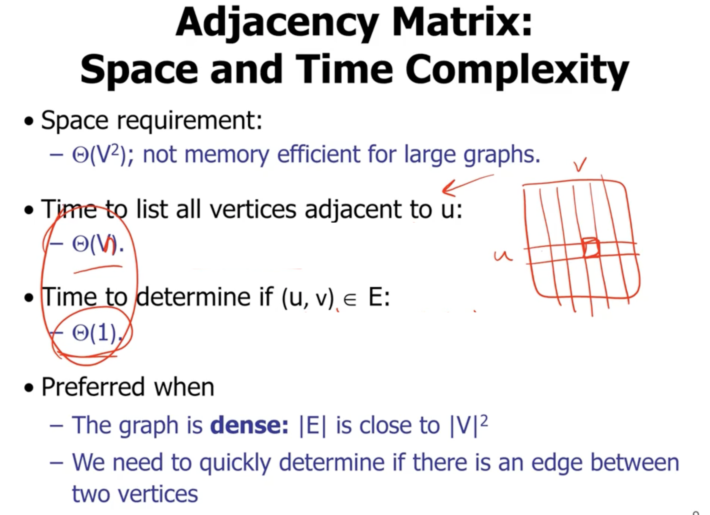
Note: In a spare graph, the adjacency list has much better space complexity.

So, generally:

• if the graph is spares, you want to use an adjacency list
• if the graph is dense, you want to use an adjacency matrix

Some examples #

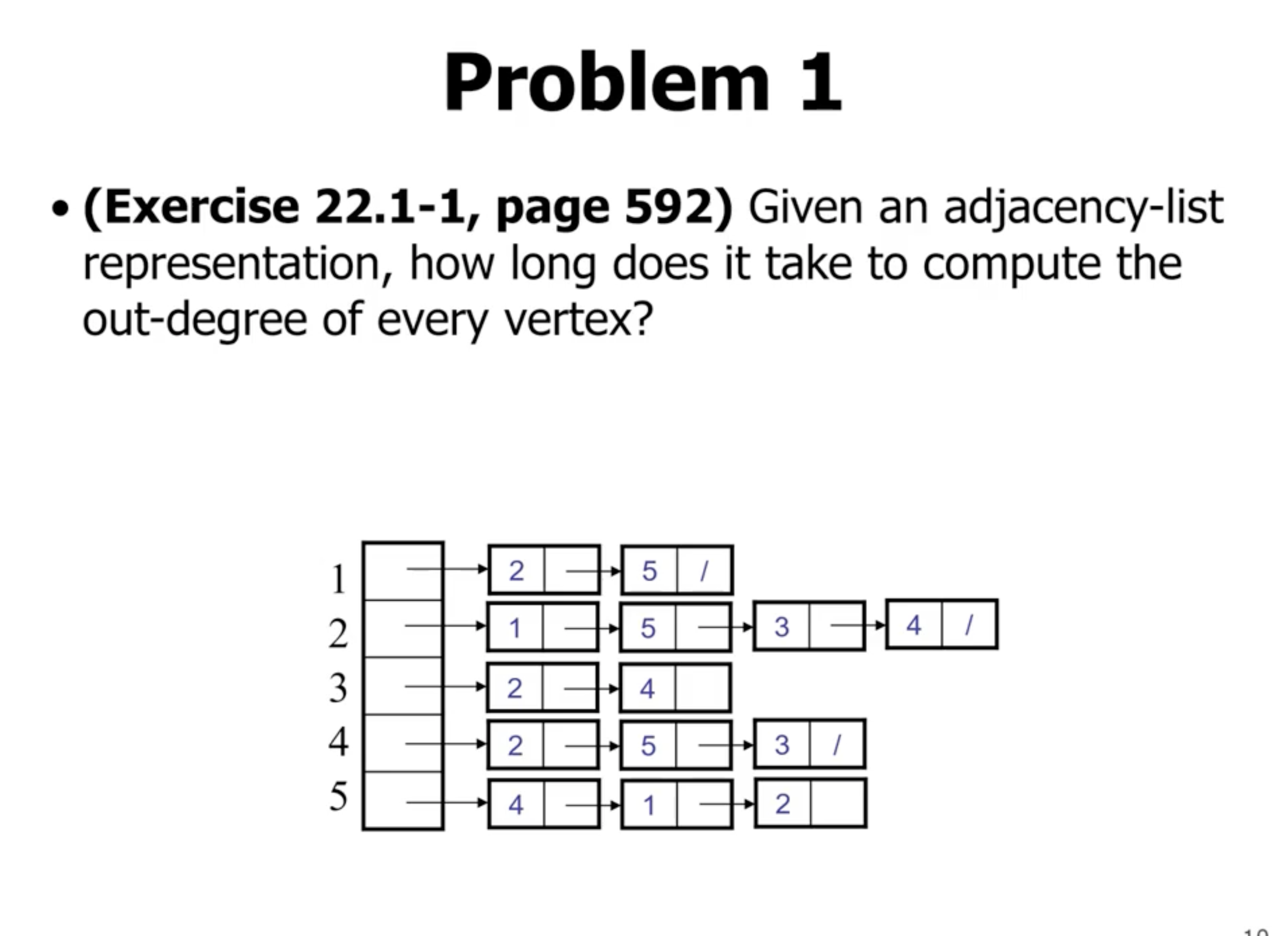
for v in vertices
    walk linked list and keep track of length
return length

This is has a runtime complexity of \( \Theta(V+E) \) .

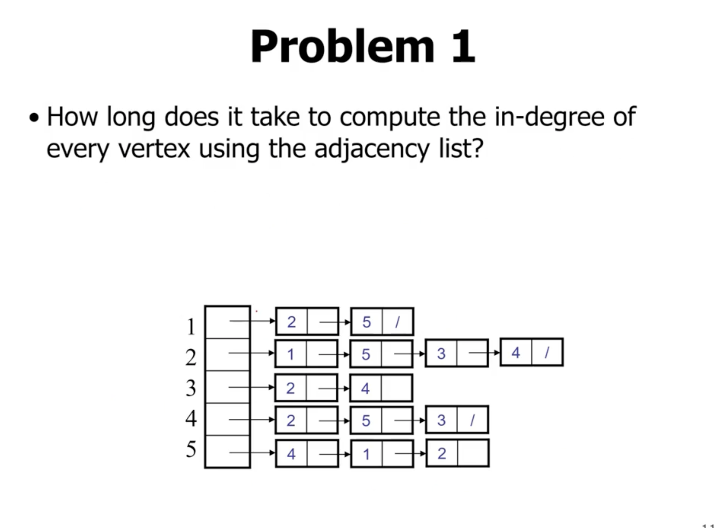
For example the in_degree(4) is 3, because it appears in the adjacency list of 3 other vertices. To calculate a single in-degree of a vertice we could do something like

in_degree(n):
    for v in vertices except n
        walk linked list
            if n appears in list, degree++
    return degree++

However, if we want the in degree of all vertices, this will have a really bad runtime complexity: \( \Theta(V(V+E)) \) .

So, it is better to calculate all of them at once.

in_degree(list):
    n = length of list
    in_degree_array[n] initialized to 0s
    for v in vertices:
        for node in linked list:
            in_degree_array[node]++
    return in_degree_array

This returns an array of values corresponding to the in degree of each vertex. So, since we only have to loop over the entire adjacency list once, we have a runtime complexity of \( \Theta(V + E) \) .

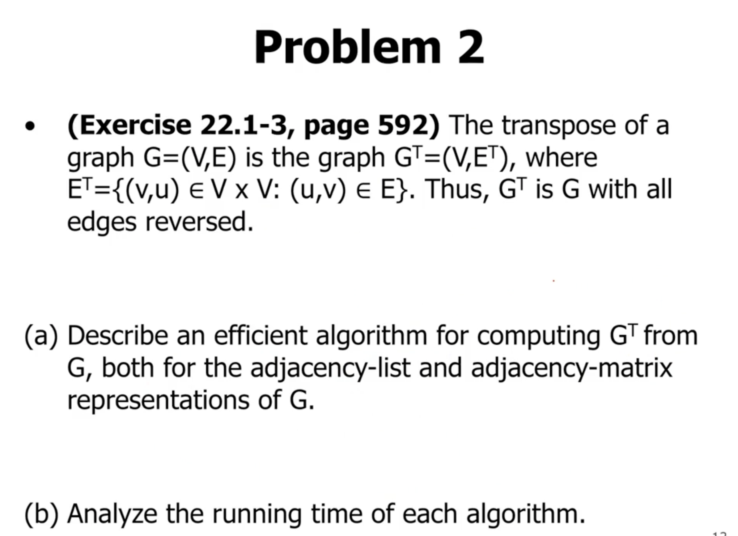
For an adjacency list #

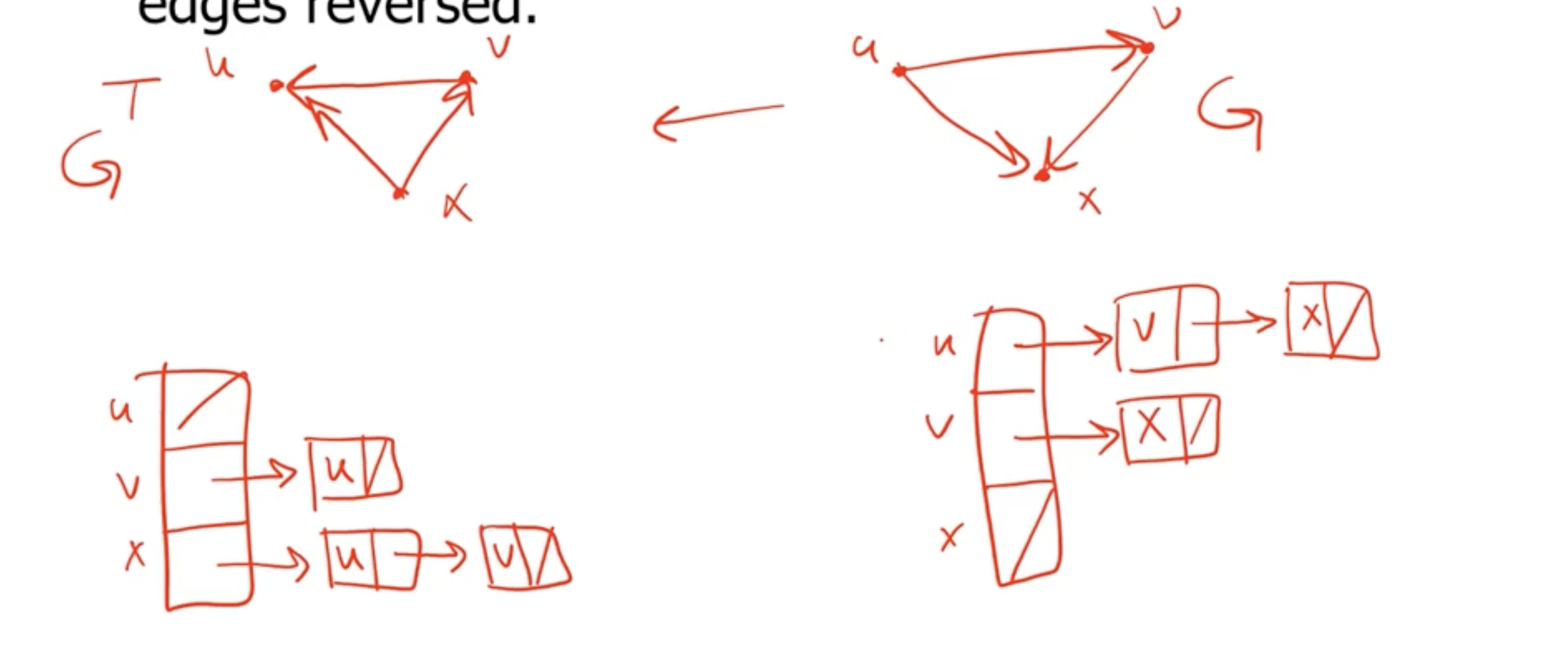
We can traverse the entire array of linked lists, and when we see a node in an adjacency list for vertex \( u \) , we can add \( u \) to the adjacency list for that node in the transposed graph.

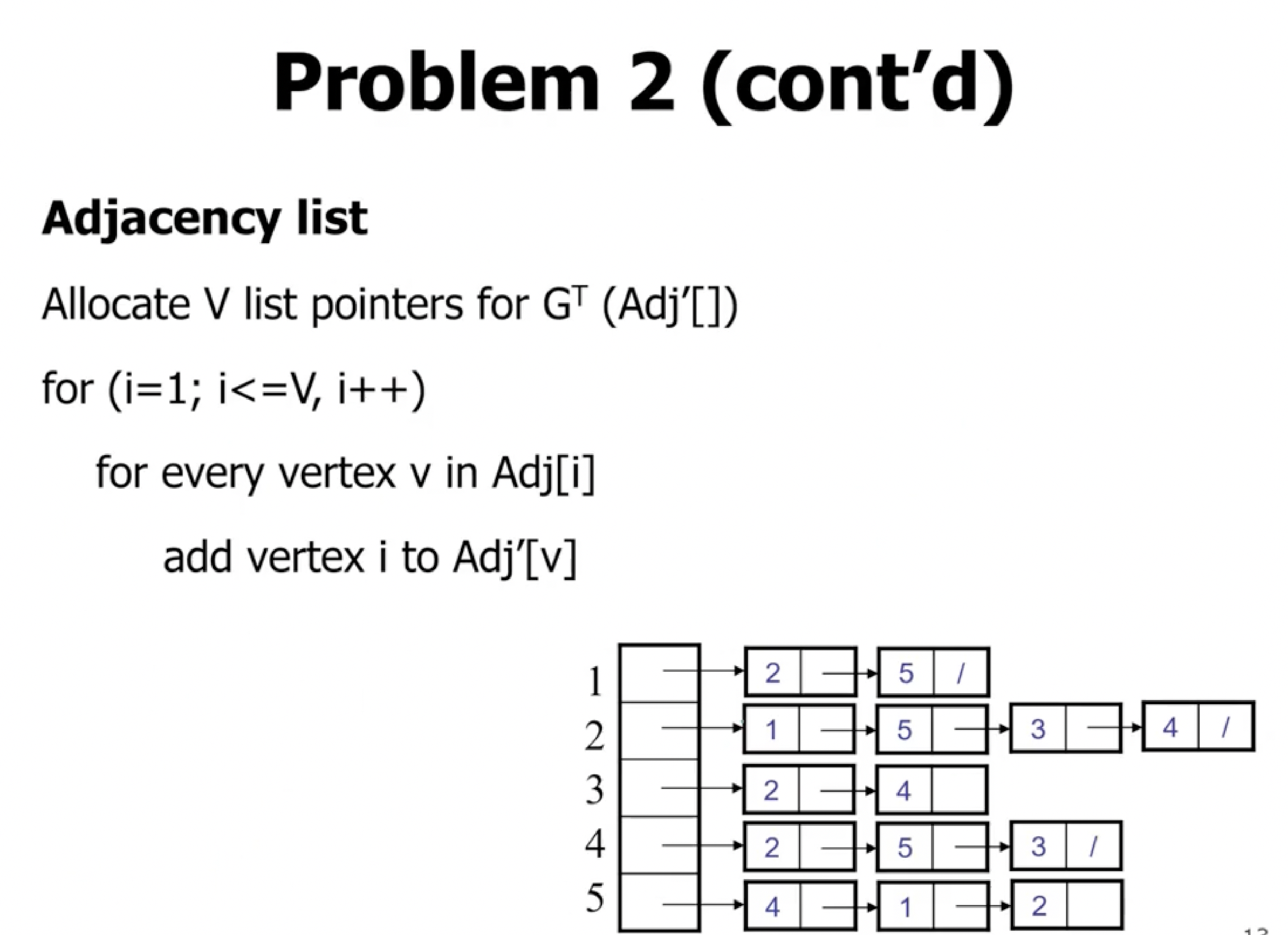
This results in a time complexity of \( \Theta(V+E) \) .

For an adjacency matrix #

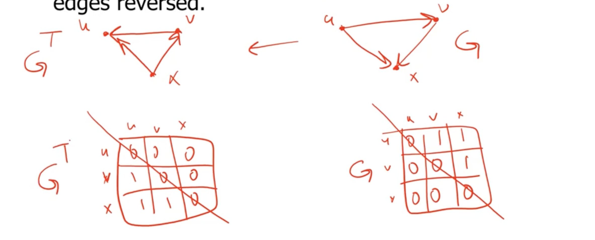
While this looks like any 0 is simply flipped to a 1, it is actually not. It is actually a mirror across the diagonal line.

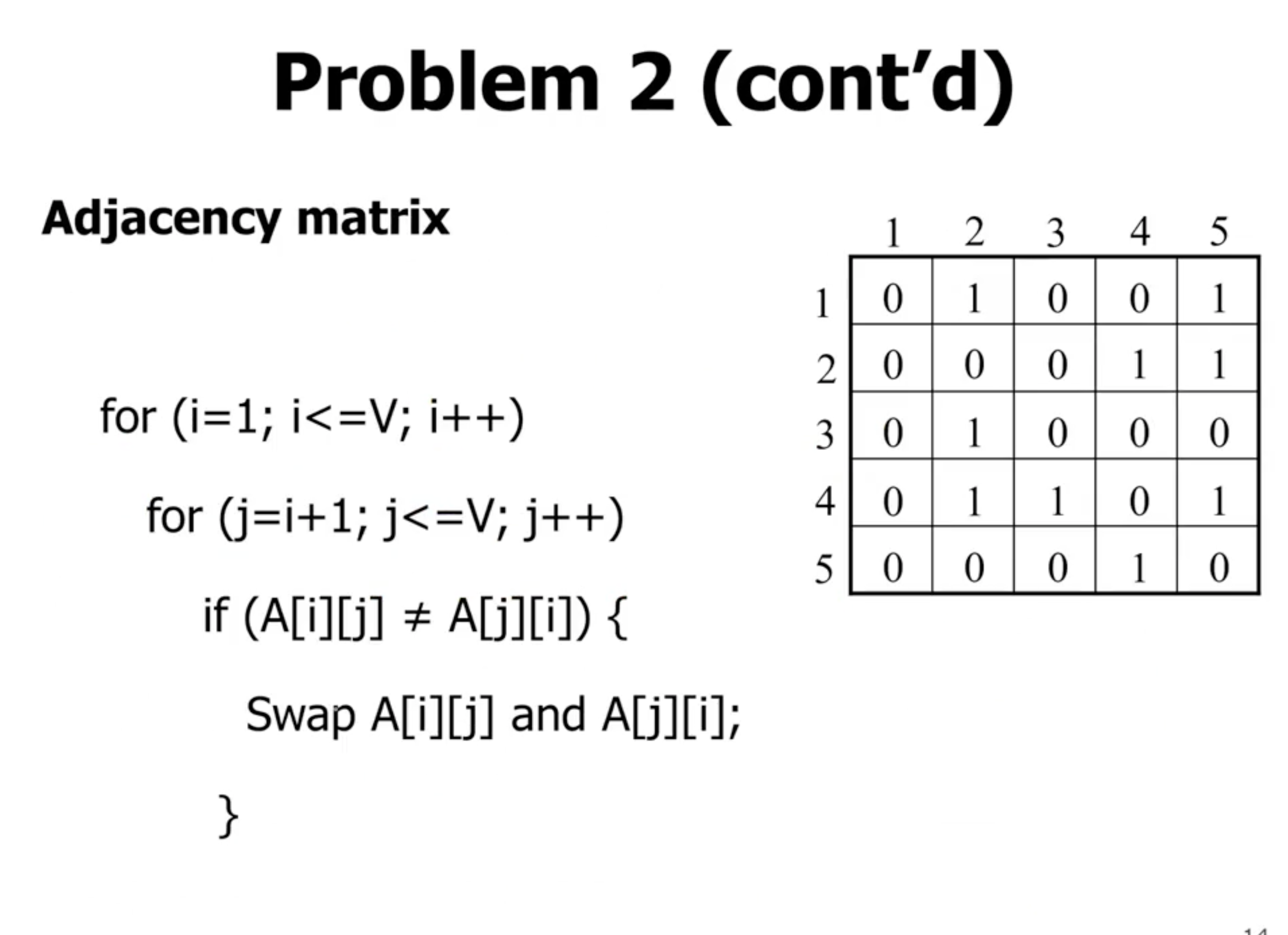
This gives a runtime complexity of \( \Theta(V^2) \) .

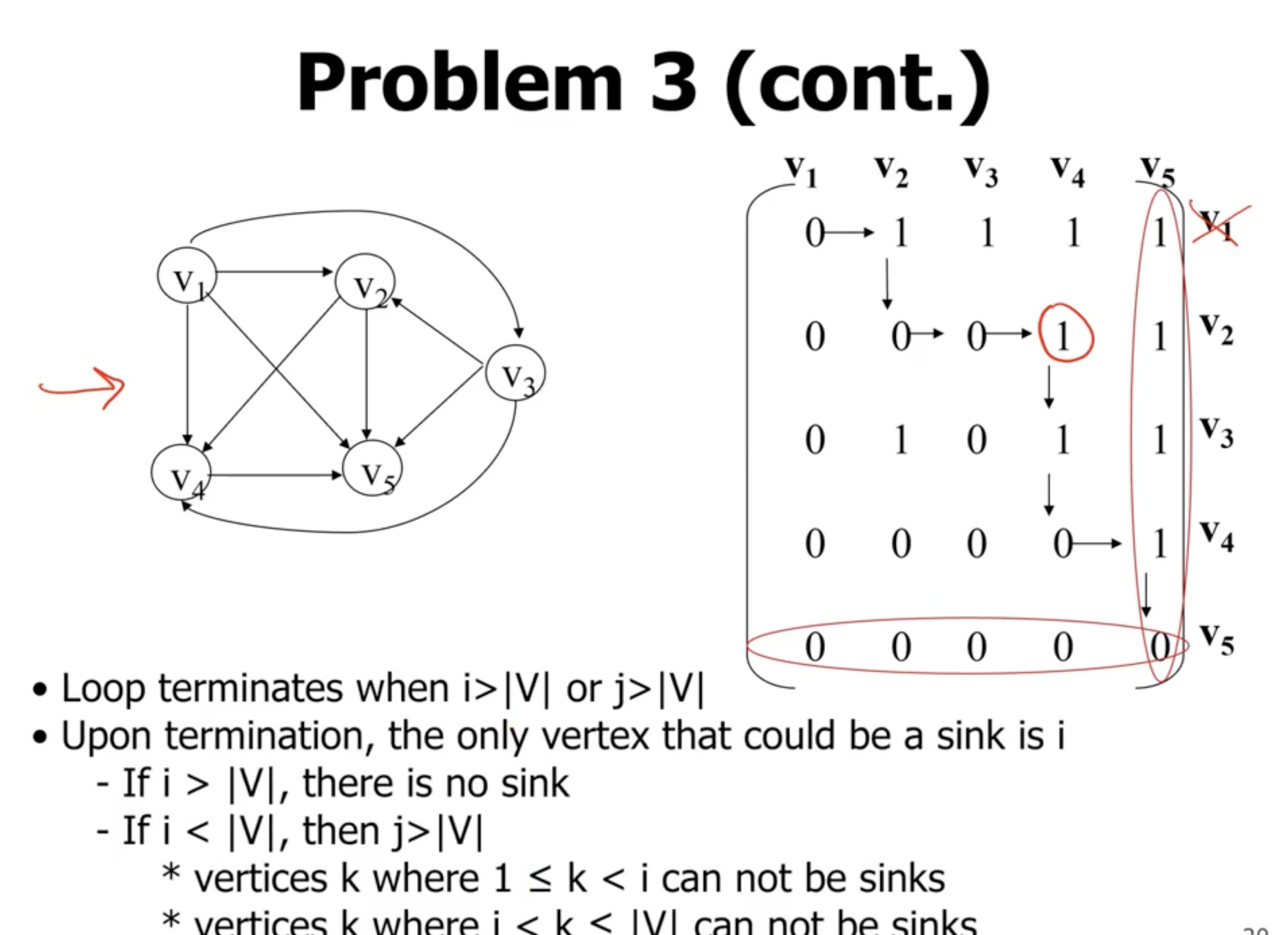
Universal sink problem #

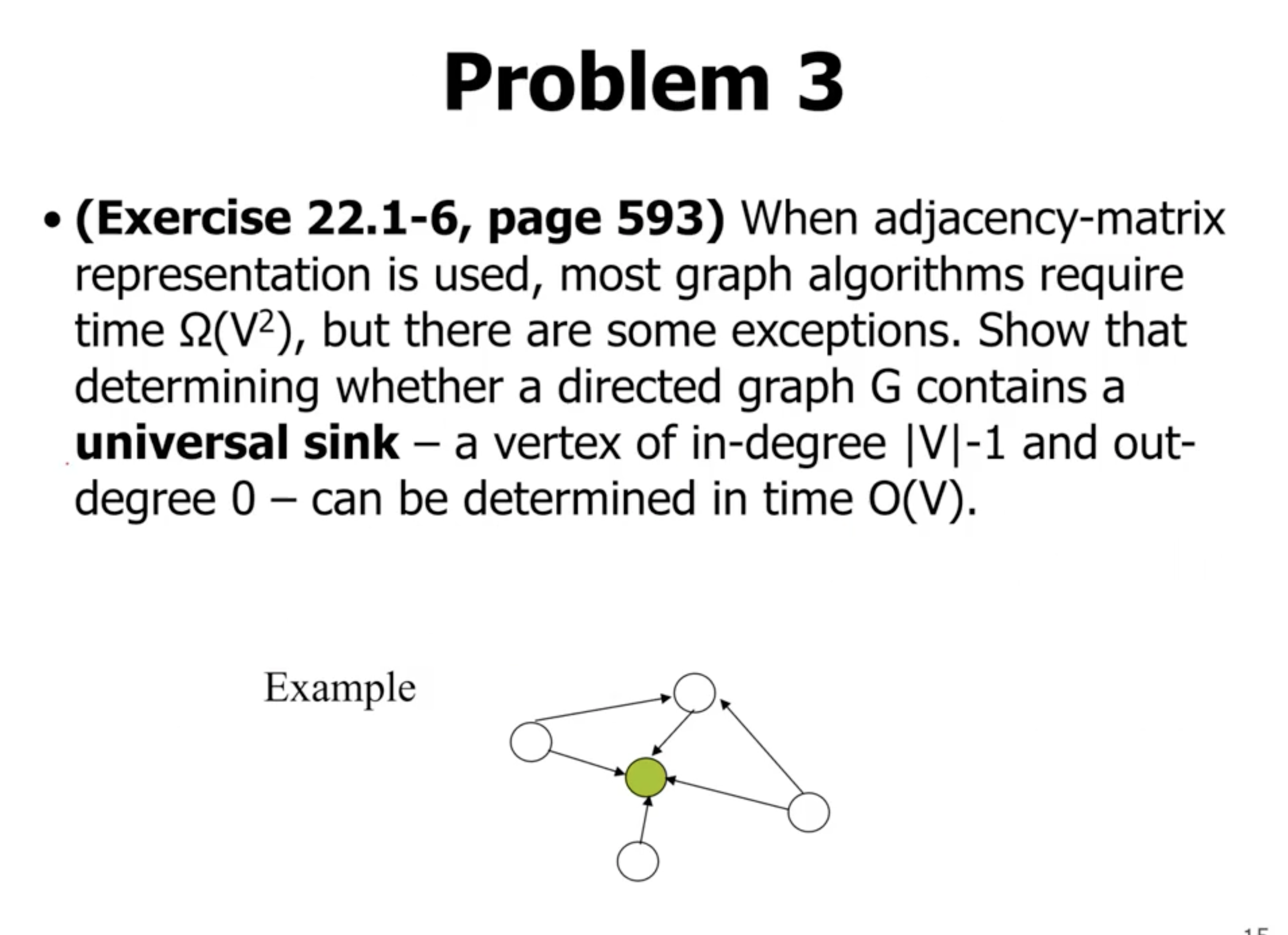
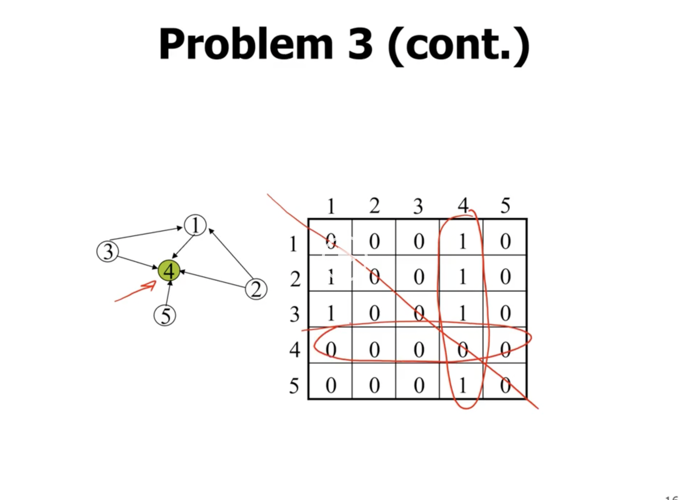
First lets answer some questions to help in the design of this algorithm:

• How many sinks could a graph have?
  • either 0 or 1
• How can we determine whether a given vertex \( u \) is a universal sink?
  • the row must contains all 0s
  • the column must contain all 1, except on the main diagonal
• How long would it take to determine whether a given vertex \( u \) is a universal sink?
  • \( O(n) \) , we check 1 row and 2 column, so \( 2n \) checks.

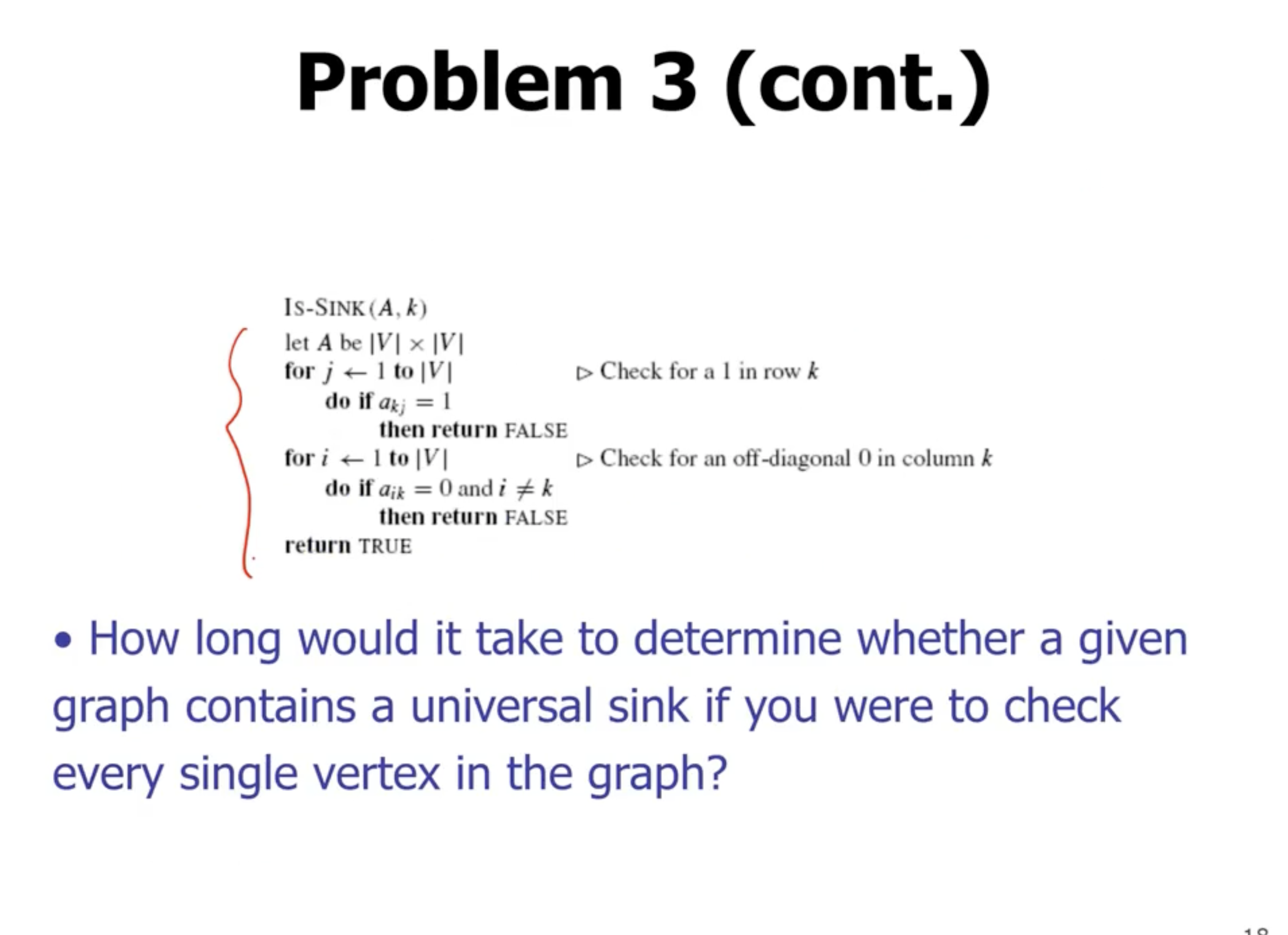
This will be \( O(v^2) \) complexity. So how can we make it better?

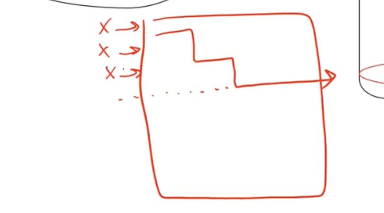
We can start at the top left of the matrix, and go to the right until we see a 1. If we see a 1, that means that the first row cannot be a universal sink, but that column with a 1 could be. So at this point we start checking down the column and make sure we keep seeing 1s. If we reach a 0 then we move to the right.

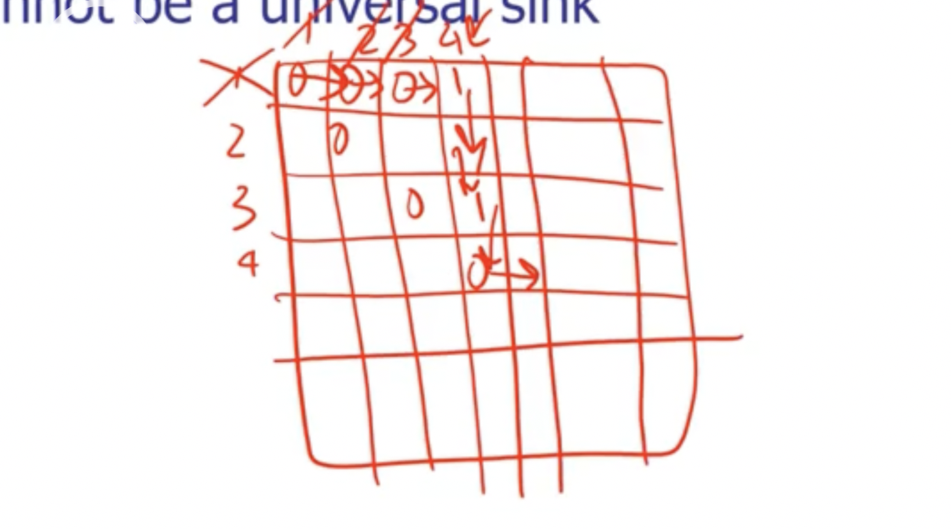
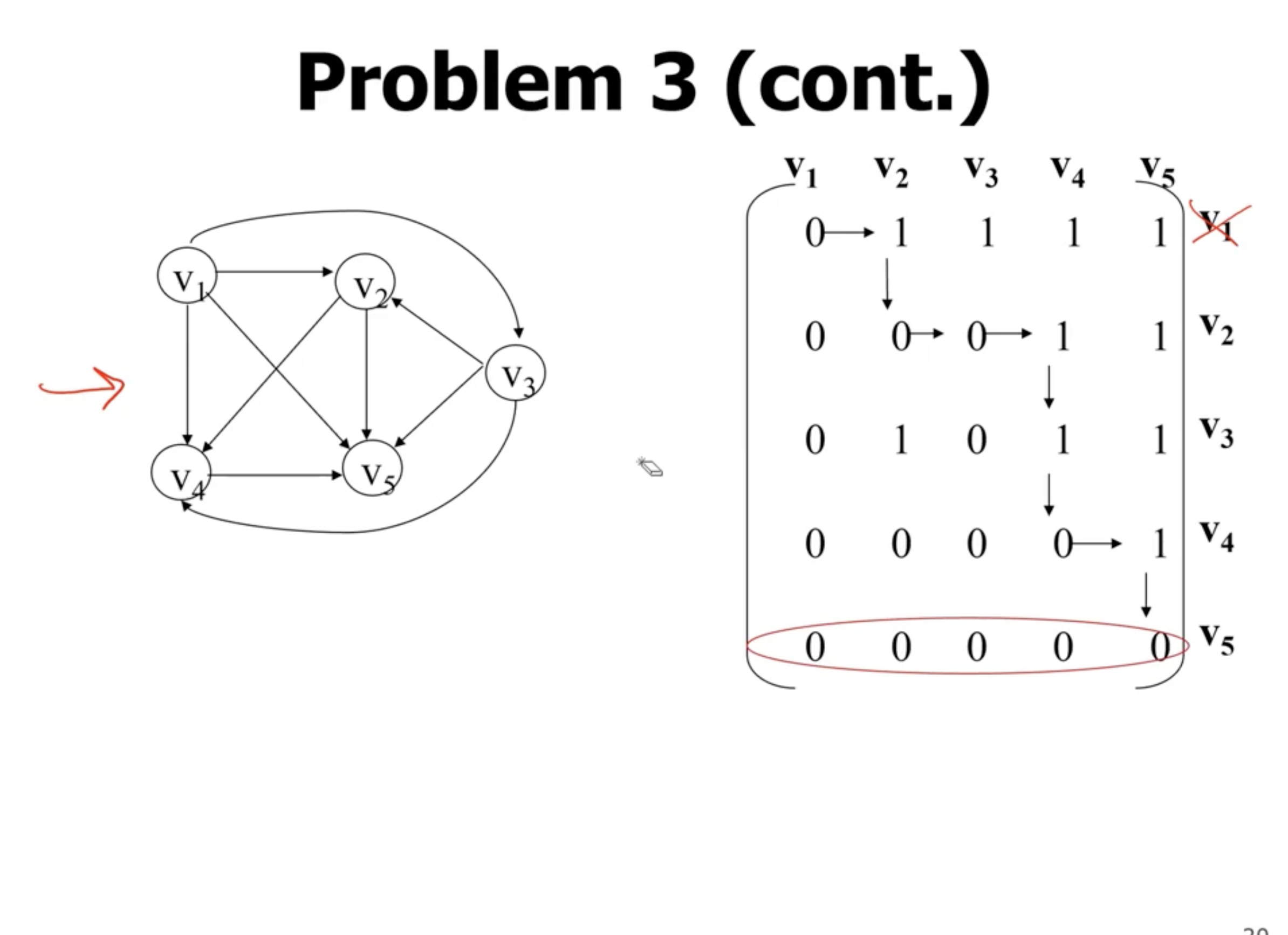
When we reach \( v_5 \) , it shows that it may potentially be a universal sink.

If at any point we leave the bounds of the matrix, the vertices before that point cannot be universal sinks.

Greedy algorithms #

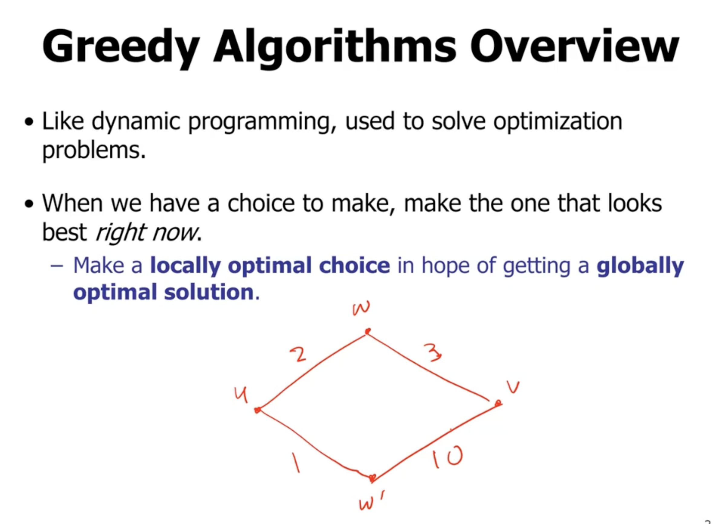
Here, in a greedy algorithm, we choose \( w' \) as the first vertex in our shortest path, because it is locally optimal.

Problems solvable via a greedy alrogithm

1. exhibit optimal substructure, meaning that a substructure of a structure is also optimal (a segment of the shortest path is optimal for that segment).
2. exhibit the greedy choice property, that is a globally optimal solution can be arrived at by making a locally optimal (greedy) choice.

Activity selection problem #

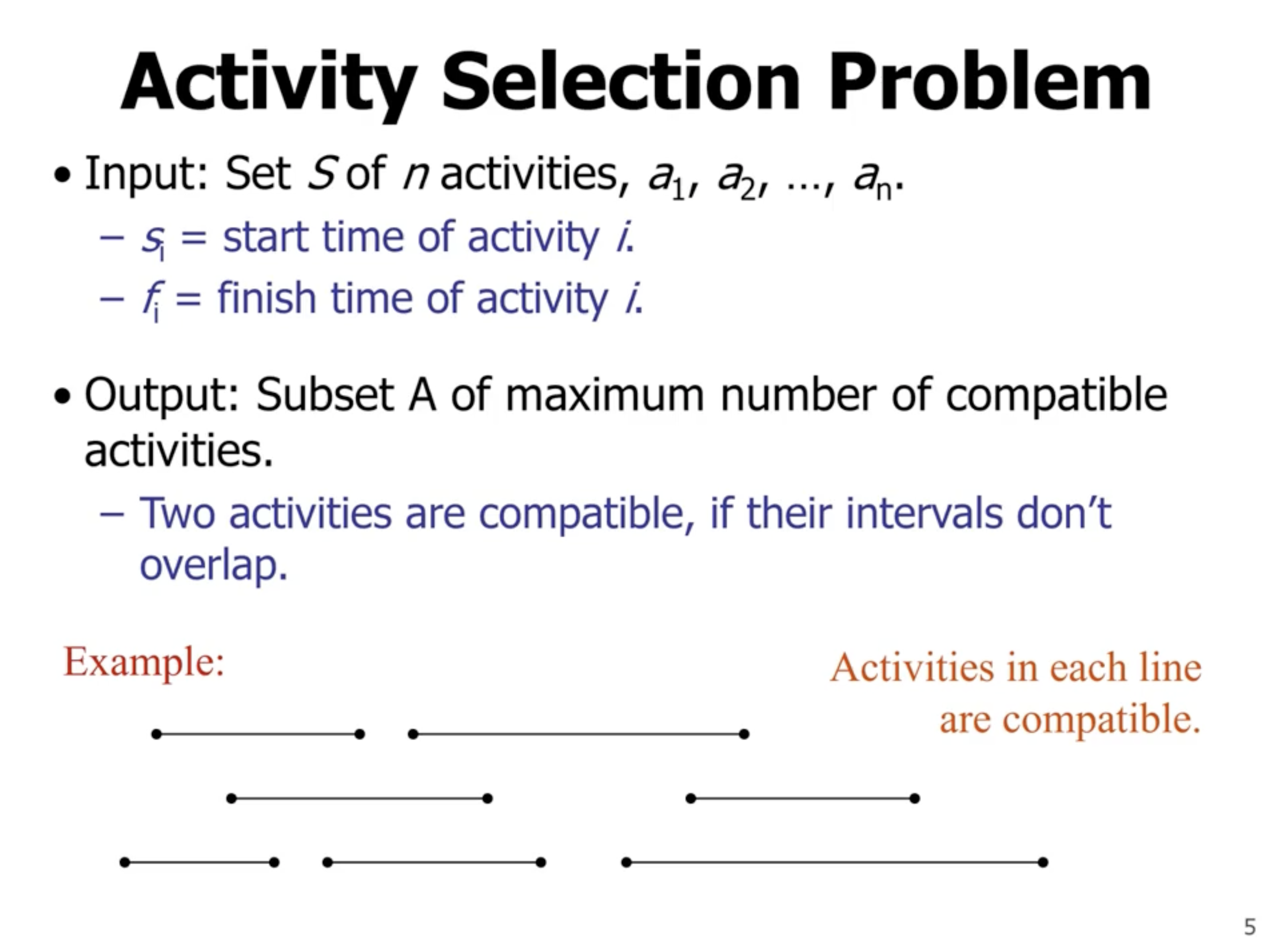
Note: This is the same as CPU scheduling.

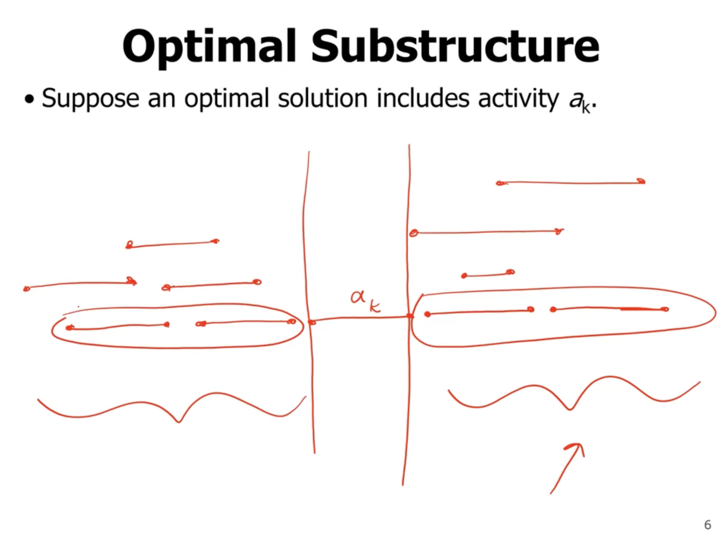
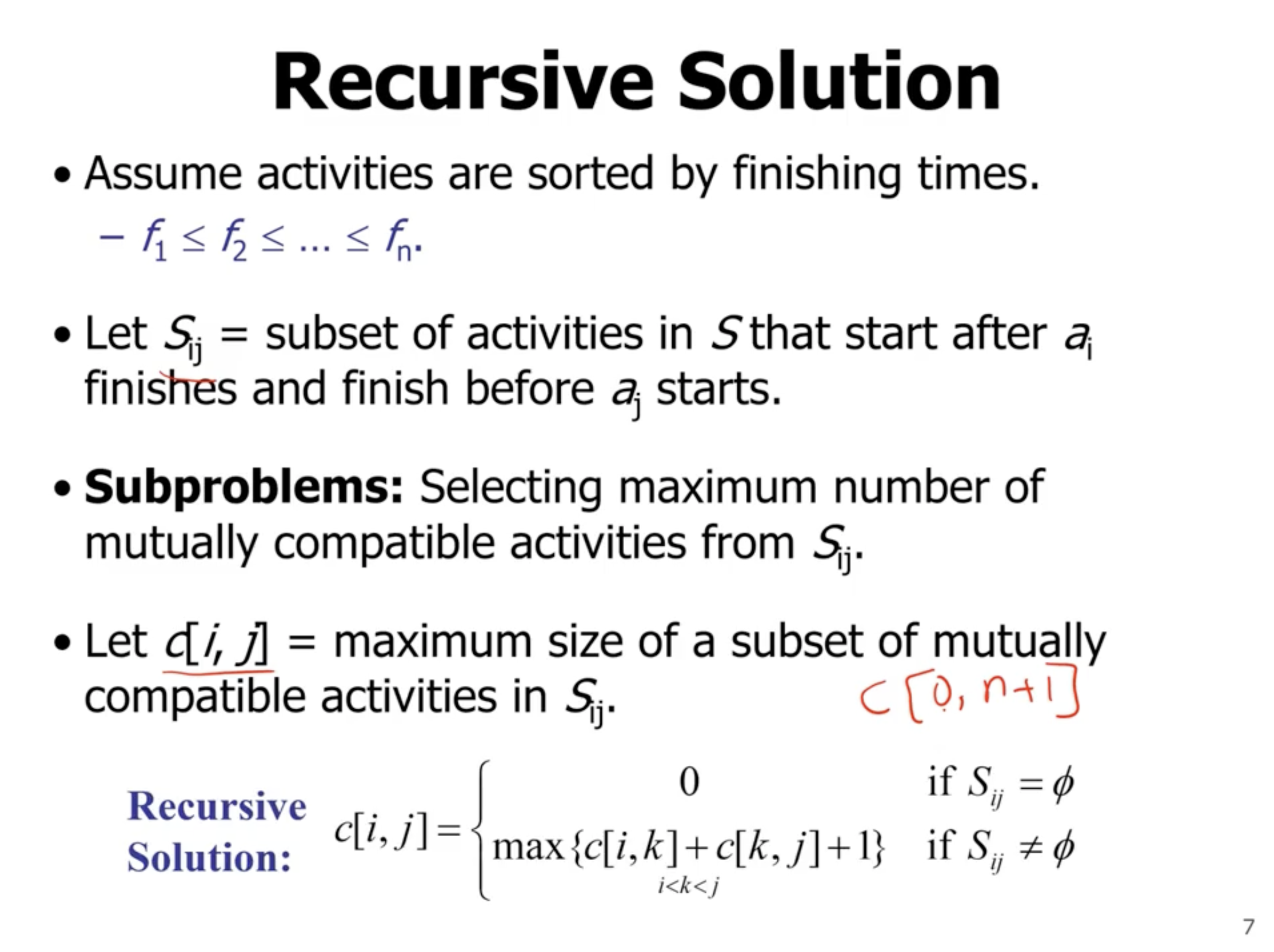
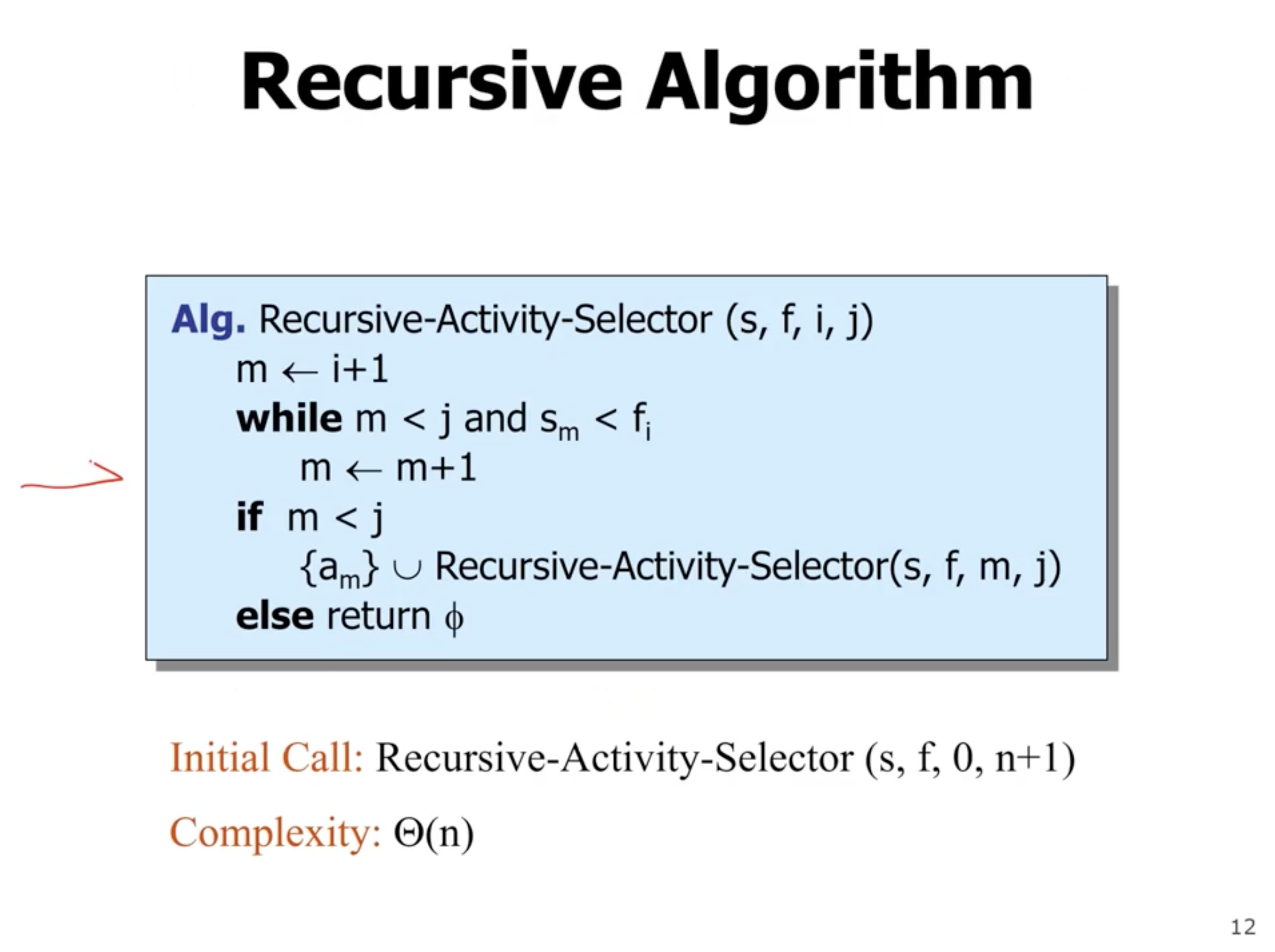
First, lets look at the recursive solution:

For the greedy algorithm, we need to define what the greedy choice is. For example, if we say that the greedy choice is the next activity to start (the shortest time between now and activity start), then it may look like this:

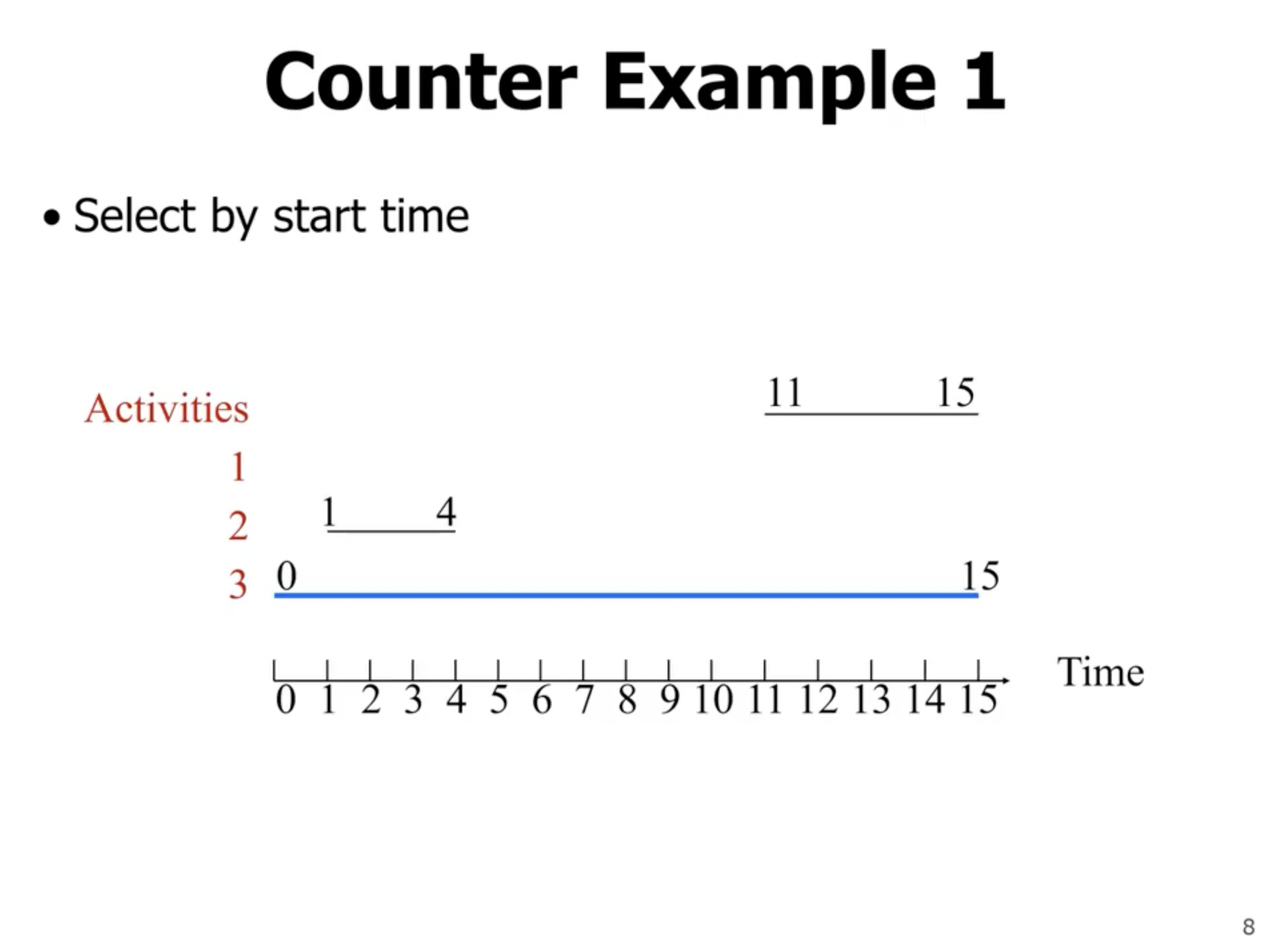
As you can see, this choice does not return the maximium number of activities we can select. So what if our greedy choice is minimum duration?

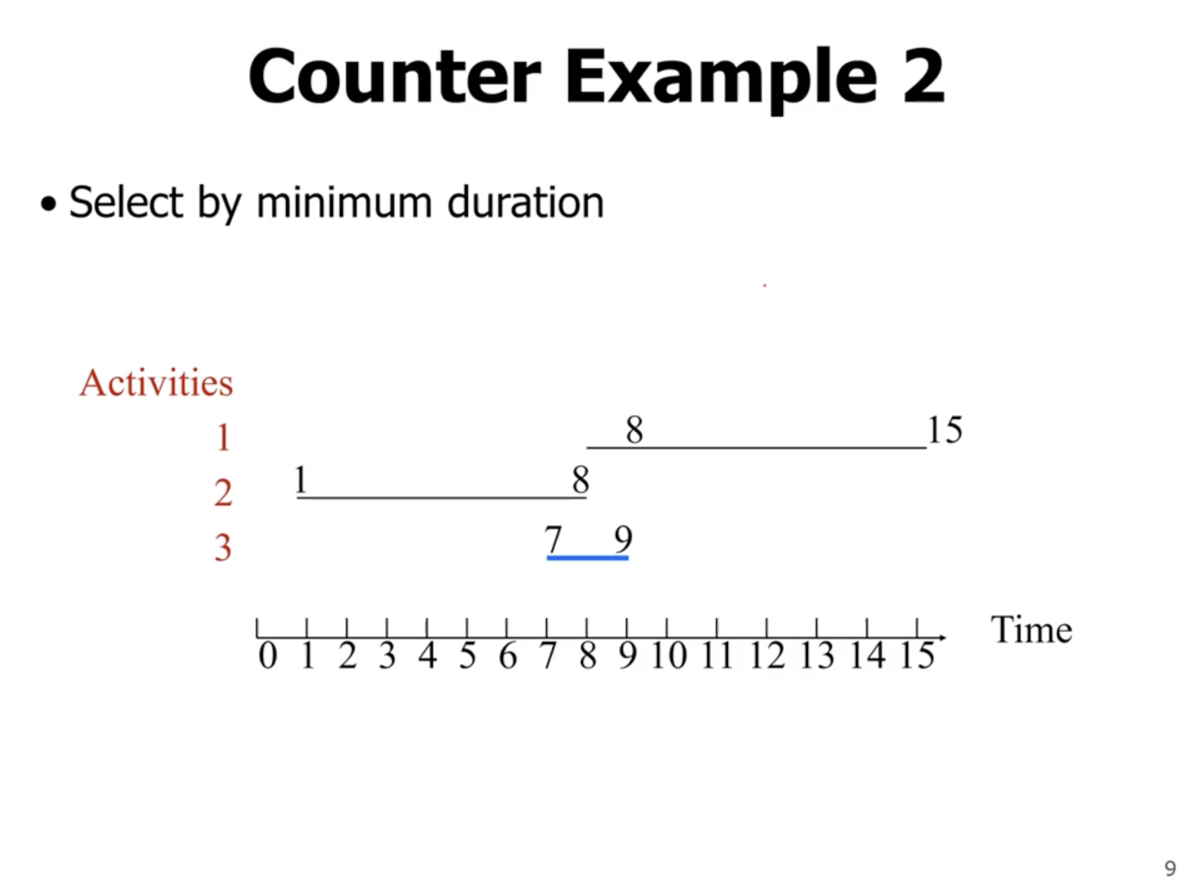
As you can see with this counter example, that doesn’t always work either.

So, what if our greedy choice is to select by fastest finishing time?

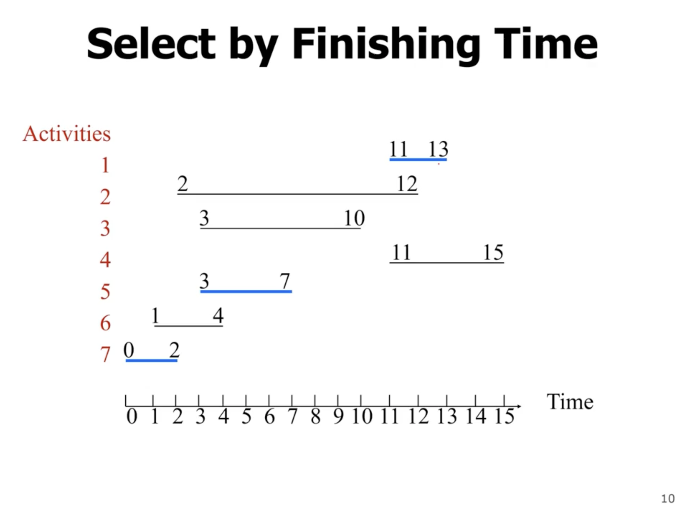
This looks like it will work. Lets show the greedy choice property:

When an activity is selected, it is selected because it finished faster than the other activities to select from. So, from this time on it will definitely be included in the optimal solution because of this property.

The knapsack problem #

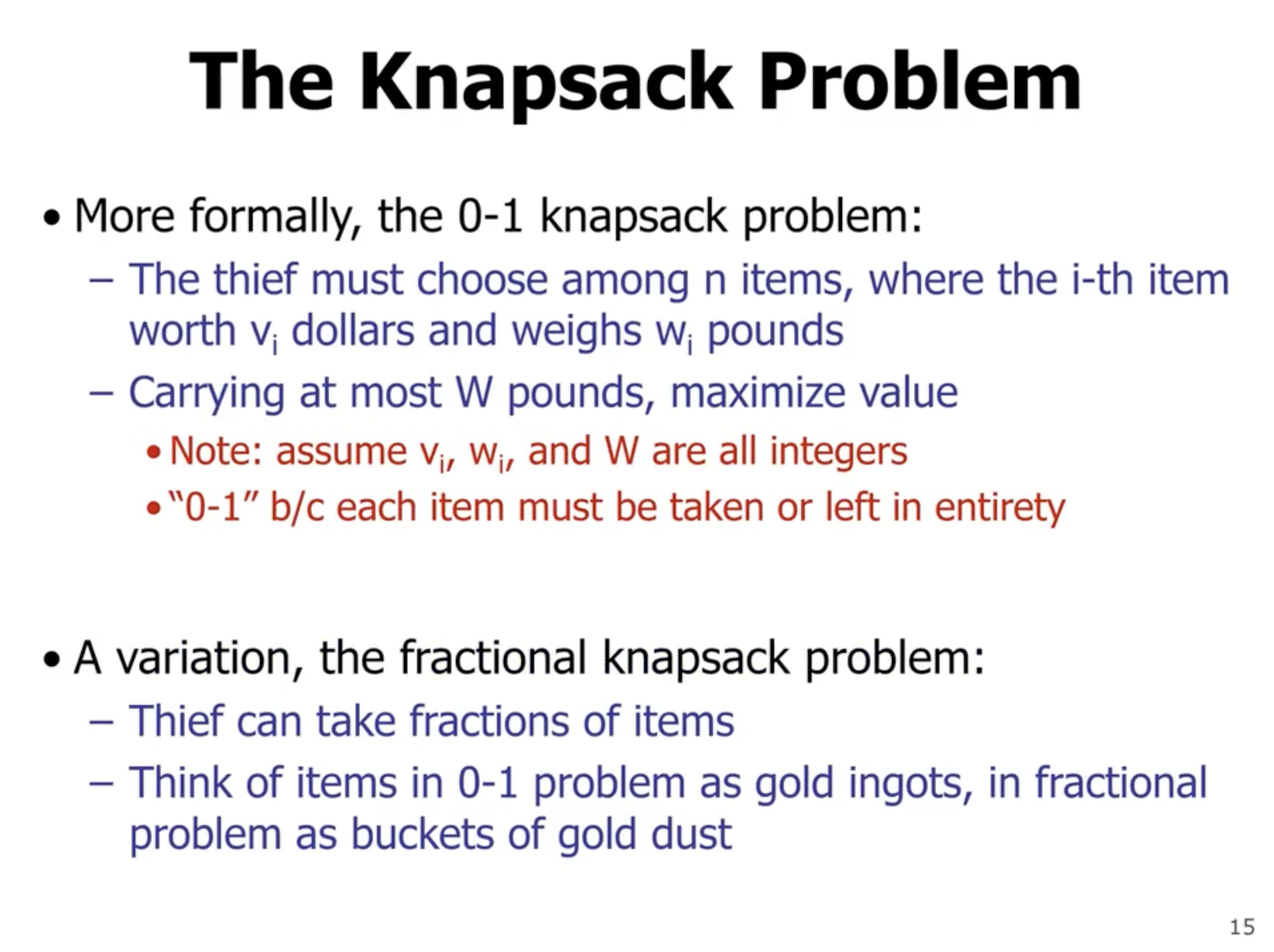
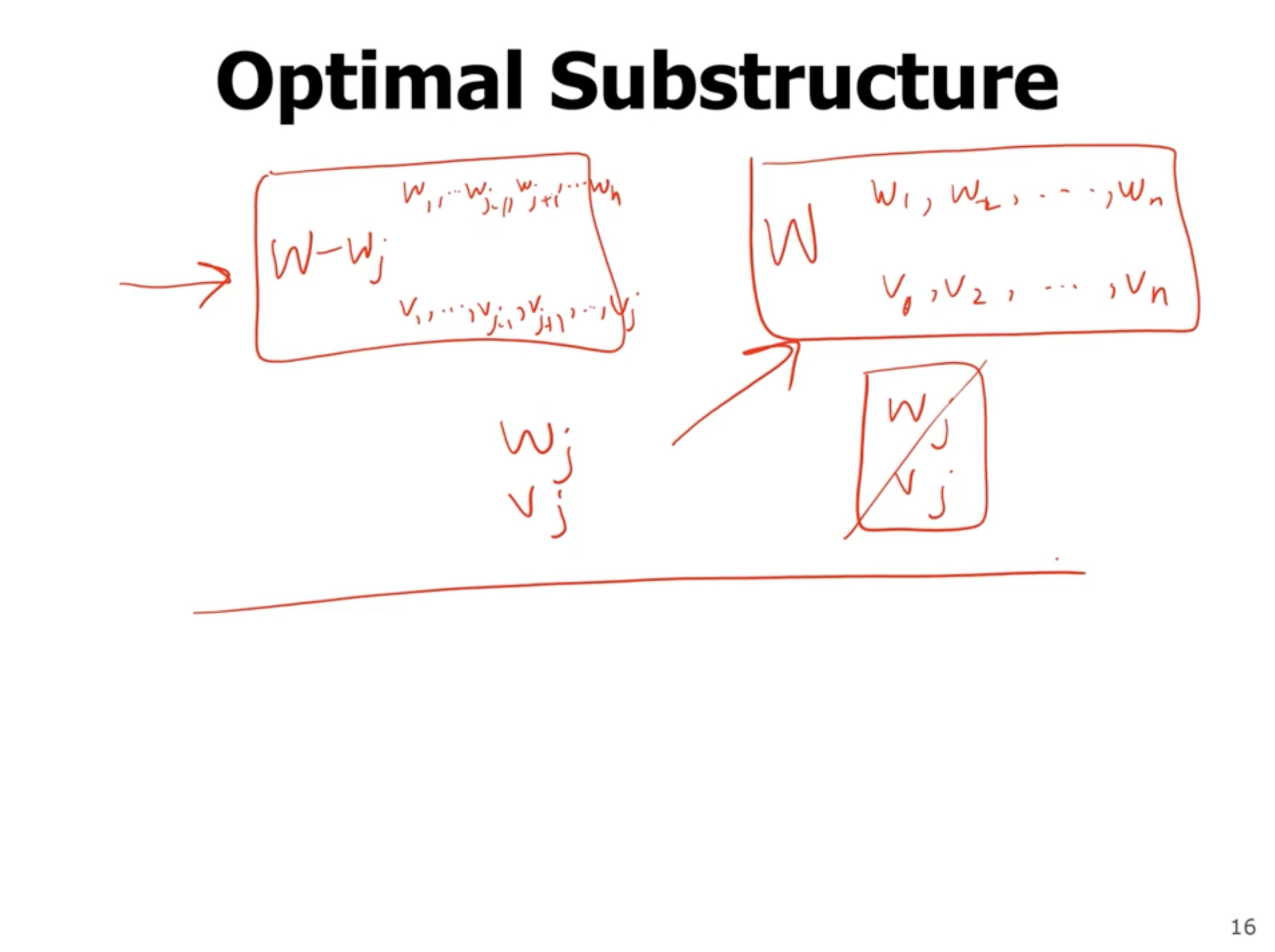
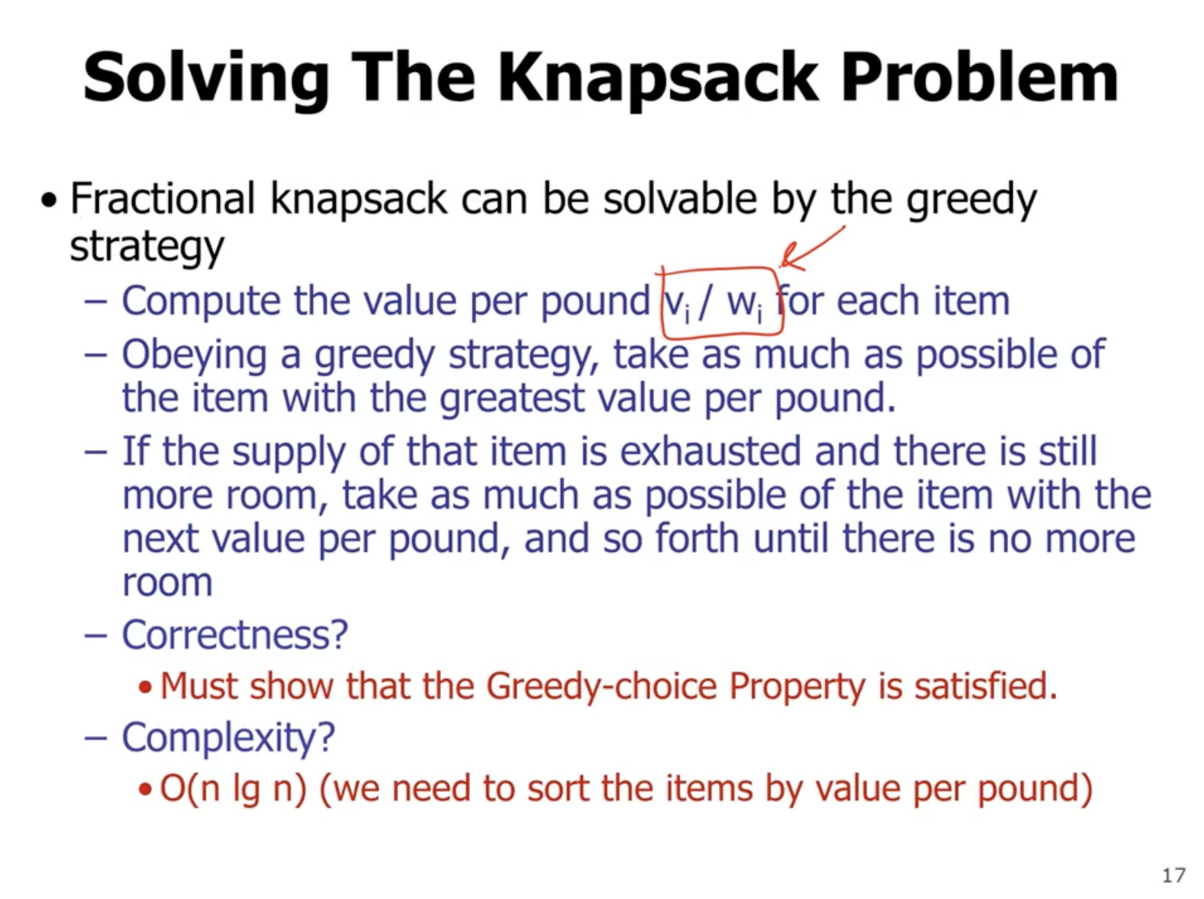
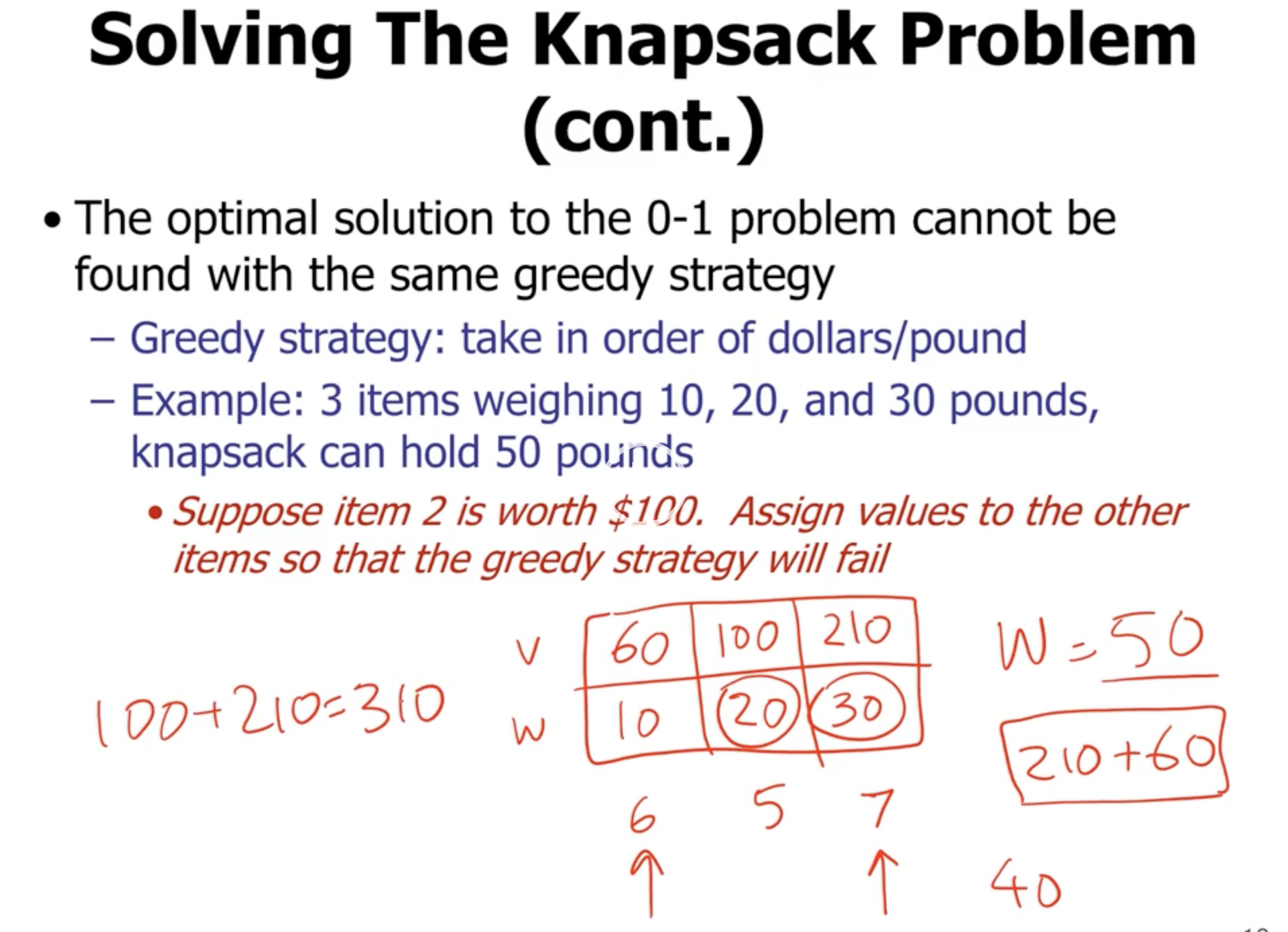
Note: The 0-1 knapsack problem can be solved by dynamic programming.