Distinguishing games #

File: Distinguishing.pdf

Cryptography used to be based on both the pedigree of the creator, and the amount of time it takes until someone can crack it. With modern cryptography, crytographers can prove that their algorithms work. The attack can be skipped if its proven that there are no weaknesses.

When we encrypt a plaintext, we want the ciphertext to look like random bits.

How do we know that the cipher is a good cipher? If an adversary can’t tell the difference between the cipher and complete random bits, then it is indistinguishable from random.

Randomness has no information in it.

To tell if the cipher is truly random looking, we can use distinguishing games:

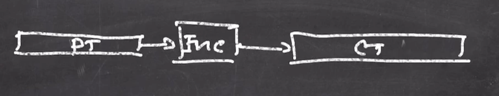
• The distinguisher (could be adversary) is given a black box, with \( A \) or \( B \) in it (equally likely).
• The distinguisher follows an algorithm and guesses \( A \) or \( B \) .

If our strategy was to always guess \( A \) , then \( \text{advantage} = 1 - 1 = 0 \) .

If our strategy was to flip a coin and guess based on the coin, then \( \text{advantage} = \frac{1}{2} - \frac{1}{2} = 0 \) .

So our distinguishing algorithm must be intelligent, it can’t simply guess.

A concrete example #

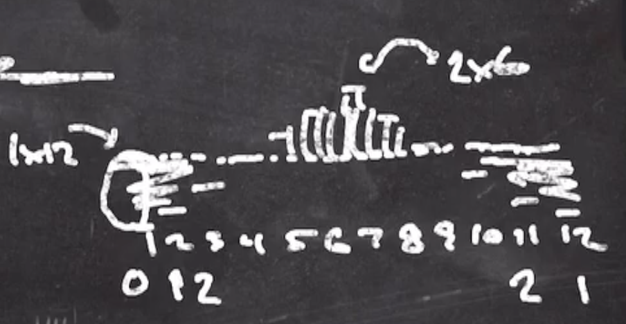
Let \( f \) be a black box with either one 12-sided die, or two 6-sided dice.

Imagine that \( f \) has a button on the side, and when we press it the die/dice are rolled, and the total is displayed to us. (We can’t tell what black box we have by looking/listening to it, we can only see the outcome.)

Also, let \( f \) be used only once, \( q = 1 \) .

To tackle this:

1. Give an algorithm using \( f \) .

x = f()
if x == 1:   // if we ever see a 1, it must be the single die
    guess "1 x 12"
else:
    guess "2 x 6"

2. Calculate the advantage

Since this is greater than 0, it is distinguishing better than just randomly guessing. We can do better however, just because we have some advantage it doesn’t necessarily mean that it is a good distinguishing algorithm.

The distribution of the outcomes for a pair of dice is:

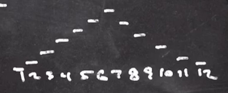
With no possibility of getting a 1.

With a 12 sided die, all outcomes are equally likely. If we overlay that on top of the pair of dice distribution:

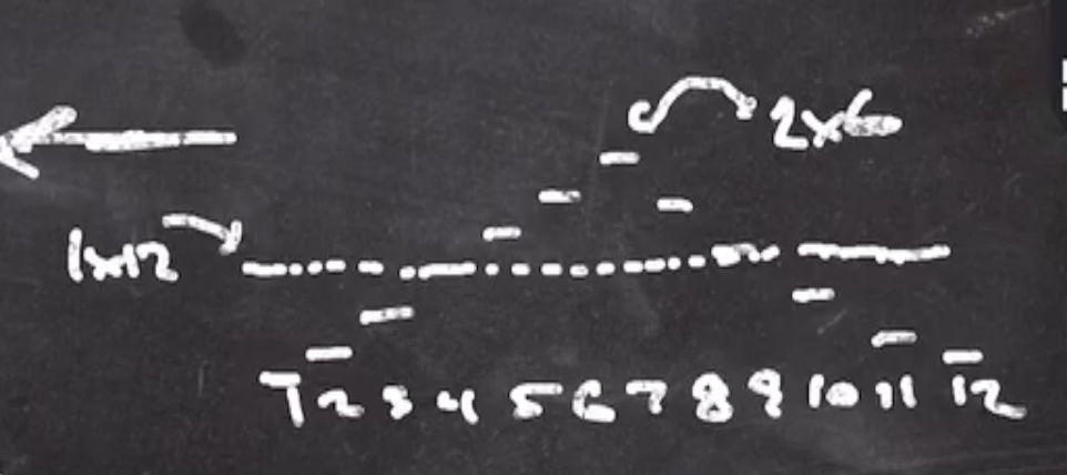
The area above the line shows that there is a better probability that the box contains 2 dice. On the ends, there is a better probability it is a single die.

So we can adjust our algorithm:

x = f()
if x in [1, 2, 3, 11, 12]:
    guess "1 x 12"
else:
    guess "2 x 6"

Note: We are leaving off the values that are the same probability for each box, ie 4 and 10.

So the new advantage is

Another example #

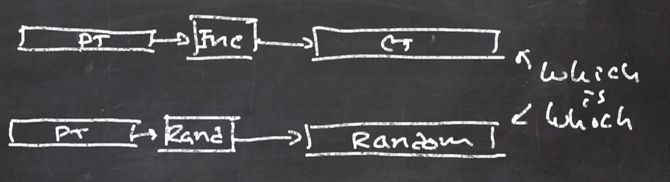
Let \( f : Z_{100} \to Z_{100} \) be either a random function or a random permutation.

The random function is fixed, and the random permutation doesn’t allow any repetition.

Let \( f \) be used only one time, \( q = 1 \) .

So what is a distinguishing algorithm? Remember the first time we invoke the random function, it will be equally likely to be any value. If its a random permutation, it’ll also give us an equally likely value (because its the first call to \( f \) ). So there is no way to distinguish them from each other, so lets set \( q = 2 \) (we can use the box twice).

If we give \( f \) 2 different inputs, and we get the same output, then it must be a random function (because permutations don’t allow repetition).

x = f(0)
y = f(1)
if x == y:
    guess "function"
else:
    guess "permutation"

Lets say we can use the black box \( q \) times.

Our distinguishing algorithm scales with \( q \) .

for i from 0 to q:
    x = f(i)
    for j from i to q:
        y = f(j)
        if x == y:
            guess "function"
else:
    guess "permutation"

Note: Sometime around the 10th (square root of \(q\)) use of the black box, we should see repetition if the box is a function (the birthday problem).

The birthday bound #

If \( q \) balls are thrown randomly into \( n \) bins, then the probability that some bin has at least two balls is roughly

This is a “cryptographer’s approximation”, it breaks down when \( q \) is large. We know that probabilities can’t be greater than 1. So this only works for small \( q \) , but it at least tells us when our probability is getting close to 1.

In cryptography, we want to keep our probabilities very close to 0, so this approximation is good enough for us, because: \( q^2 \) should never get close to \( n \) .

This is a good rough approximation for the probability that you have collisions amongst \( q \) random values coming from the codomain of size \( n \) .