MATLAB #

An introduction #

File: m170-matlab-linprog.pdf

For example, lets define a vector

x = [1 2 3]

If we want to transpose x, we can use the ':

x'

Or we can define a column vector like:

y=[1
2
3]

which can also be defined with ;:

y=[1;2;3]

So, to define an entire matrix we can use a combination of both:

A=[1 2 3; 4 5 6; 7 8 9]

We can do some matrix multiplication:

A*y

Or find the inverse:

inv(A)

We can change the format to rational numbers with:

format rat

linprog function #

For a minimization LPP with “ \( \leq \) ” and “ \( = \) ” constraints, we can directly apply the linprog function.

Given \( z = c_0 + c_1 x_1 + c_2 x_2 + \cdots + c_n x_n \) , we can put this in a vector of coefficients:

and a vector of our decision variables

we can describe this as

So,

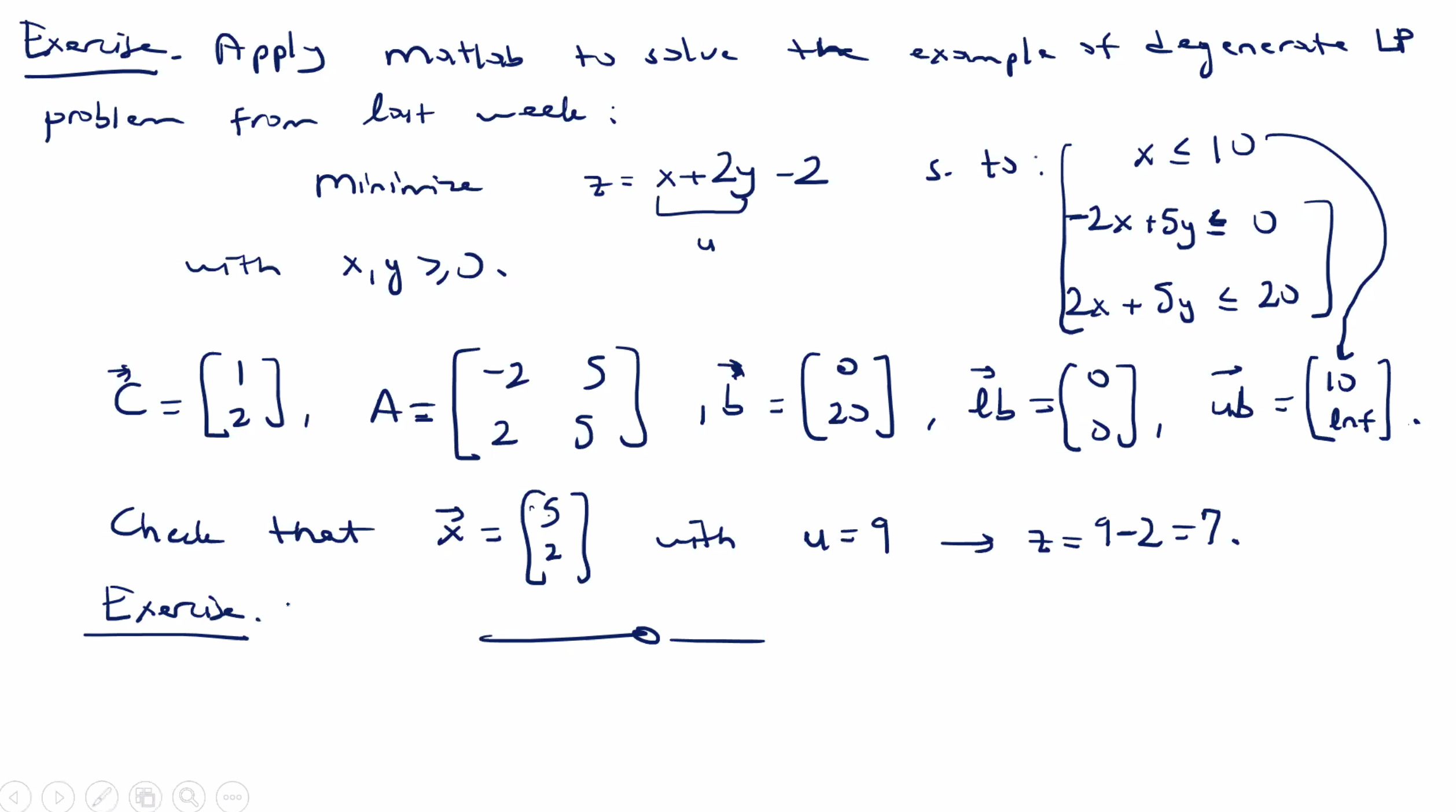
1. We minimize \( u = \sum_{k=1}^{n} c_k x_k \) , subject to the same constraints.
2. Convert all constraints to “ \( \leq \) ” or “ \( = \) ”.

Note on notation: if we say \( \bar{x} \leq \bar{y} \) , then that means for each \( k \) , \( x_k \leq y_k \) .

For “ \( \leq \) ” constraints:

For “ \( = \) ” constraints:

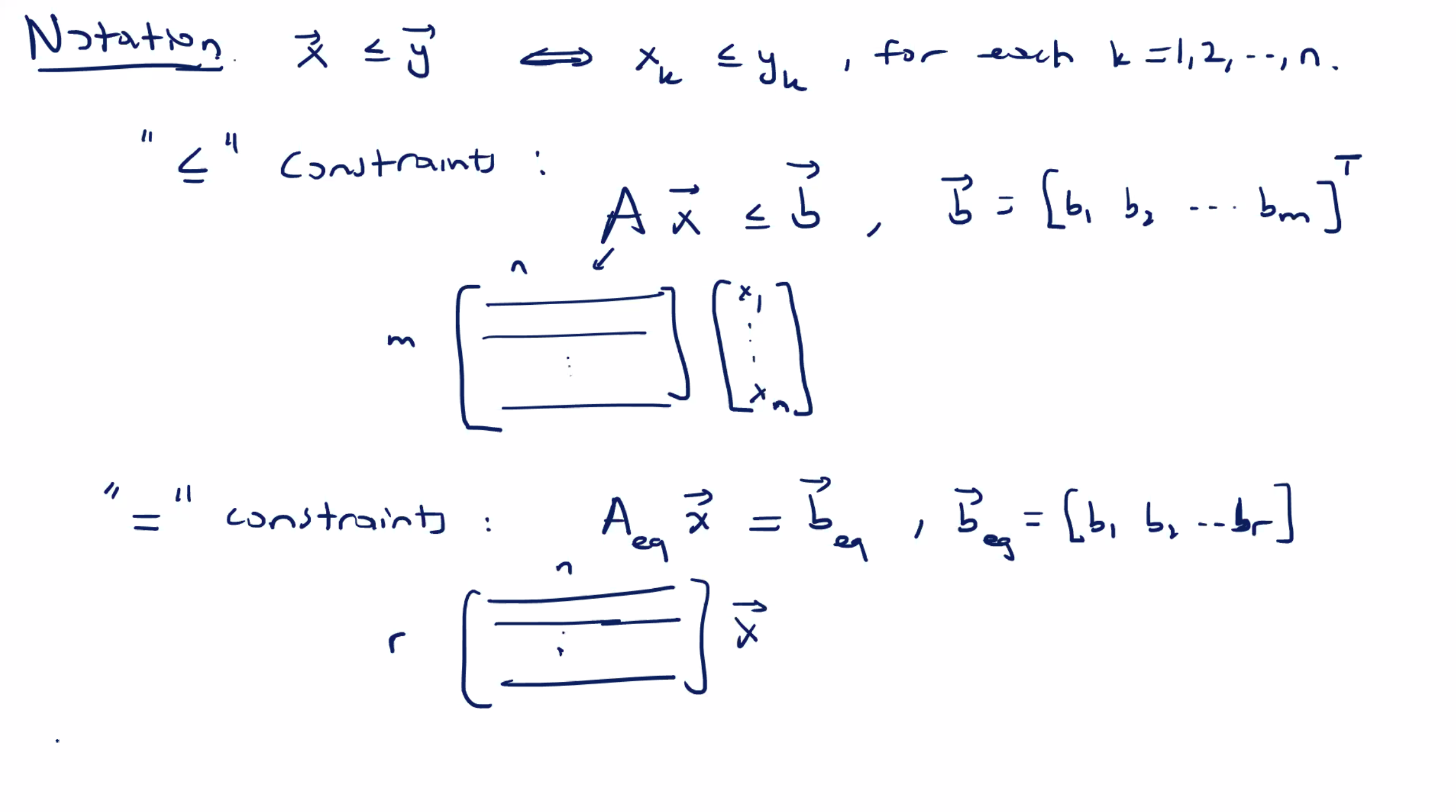
For upper and lower bounds: \[\begin{aligned} \bar{\text{lb}} \leq \bar{x} \leq \bar{\text{ub}} \end{aligned}\]

where \( \text{lb} \) is lower bound, and \( \text{ub} \) is upper bound.

So to minimize \( u = c^T \bar{x} \) subject to \[\begin{aligned} A \bar{x} &\leq \bar{b} \\ A_\text{eq} \bar{x} &= \bar{b}_\text{eq} \\ \text{lb} &\leq \bar{x} \leq \text{ub} \end{aligned}\]

We use this in the linprog function like so:

x = linprog(c, A, b, Aeq, beq, lb, ub)

which will return the optimal solution. If we are also interested in the u value, we can call the function like this:

[x,u] = linprog(c, A, b, Aeq, beq, lb, ub)

where x is the optimal solution, and u is the optimal value (minimal).

If we are missing a parameter, like ub, we can replace it with a [].

A concrete example #

Minimize \( z = 1 + x_1 - x_2 + 2x_3 \) subject to \[\begin{aligned} -x_1 + x_2 + x_3 &\geq 5 \\ 2x_1 - 2x_2 + x_3 &\leq 5 \\ x_2 - x_3 &= 1 \end{aligned}\]

and \( x_k > 0 \) , for each \( k \) .

So even though this is in canonical form, we need to change the first constraint to either an \( = \) or \( \leq \) constraint. Then, we need to identify our coefficient vector \( c \) .

So our new constraint is obtained by multiplying both sides by \( -1 \) .

Let \( u = x_1 - x_2 + 2x_3 \) , where we can take the coefficients to get \( c^T = \begin{bmatrix} 1&-1&2 \end{bmatrix} \) .

To get \( A \) , we can use the coefficients of the constraints:

\( A \bar{x} = \begin{bmatrix} 1 & -1 & -1 \\2 & -2 & 1 \end{bmatrix} \) and \( \bar{b} = \begin{bmatrix} -5 \\ 5 \end{bmatrix} \)

Our equality constraint is \( x_2 - x_3 = 1 \) , so \( \begin{bmatrix} 0 & 1 & -1 \end{bmatrix} \bar{x} = 1 \) .

So \( A_\text{eq} = \begin{bmatrix} 0 & 1 & -1 \end{bmatrix} \) and \( b_\text{eq} = [1] \) .

We only have a lower bound (the sign constraints), so \( \text{lb} = \bar{0} \) , and our upper bound is infinity.

So now that we have identified all necessary parameters, we can enter into MATLAB and then into the linprog function:

C=[1 -1 2]'
A=[1 -1 -1; 2 -2 1]
b=[-5; 5]
Aeq=[0 1 -1]
beq=[1]
lb=[0 0 0]'

[x,u] = linprog(C, A, b, Aeq, beq, lb, [])

which returns

Optimal solution found.

x =
    0
    3
    2
u =
    1

So our minimal value is \( z = 1 + u = 1 + 1 = 2 \) with \( x_1 = 0, x_2 = 3 \) and \( x_3 = 2 \) being the optimal values of decision variables.

Another example #

If we want to use linprog for a maximization problem, we need to convert it to a minimization problem. Minimizing \( z \) is the same as maximizing \( -z \) .

Maximize \( z = 7x_1 + 6x_2 \) subject to

And positive sign constraints.

To use linprog, we consider minimizing \( -z = u = -7x_1 - 6x_2 \) .

C=[-7 -6]'
A=[2 1; 1 4]
b=[3;4]
lb=[0 0]'

[x,u] = linprog(C, A, b, [], [], lb, [])

which returns

Optimal solution found.

x =
    8/7
    5/7

u =
    -86/7

Then, the solution to the original (max) problem is \( z = \frac{86}{7} \) , with \( x_1 = \frac{8}{7} \) and \( x_2 = \frac{5}{7} \) .

A more involved example #

Minimize \( z = 3x_1 + 2x_2 \) subject to \[\begin{aligned} -x_1 + 2x_2 &\leq 40 \\ x_1 + 2x_2 &\geq 40 \to -x_1 - 2x_2 \leq 40 \\ x_1 &\geq 10 \to -x_1 \leq -10 \\ 0 \leq x_2 &\leq 30 \end{aligned}\]

We can use the upper bound of \( x_2 \) in the \( \bar{b} \) matrix, but leave the lower bound in the lower bound vector.

So, we could have \( \bar{C} = \begin{bmatrix} 3\\2 \end{bmatrix} \) , and \( A=\begin{bmatrix} -1 & 2 \\ -1 & -2 \end{bmatrix} \) .

Our right hand side vector is \( \bar{b} = \begin{bmatrix} 40 \\-40 \end{bmatrix} \) .

Our lower bound vector is \( \text{lb} = \begin{bmatrix} 10\\0 \end{bmatrix} \) and upper bound vector is \( \text{ub} = \begin{bmatrix} \infty \\30 \end{bmatrix} \)

So, in MATLAB:

C=[3 2]'
A=[-1 2;-1 -2]
b=[40 -40]'
lb=[10 0]'
ub=[inf 30]'

[x, u] = linprog(C, A, b, [], [], lb, ub)

which returns

Optimal solution found.

x =
    10
    15

u =
    60