Sensitivity analysis cont. #

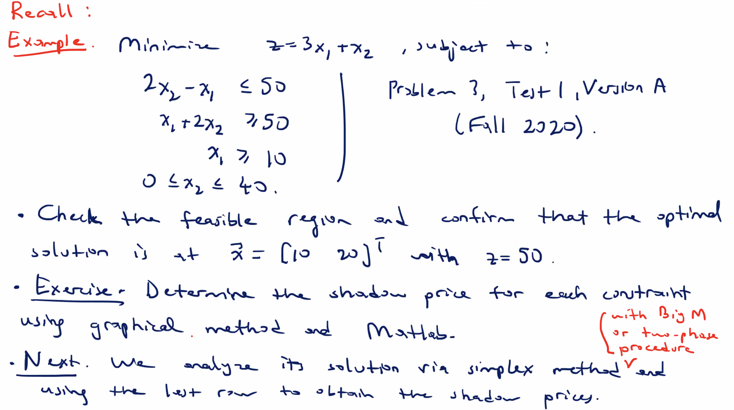
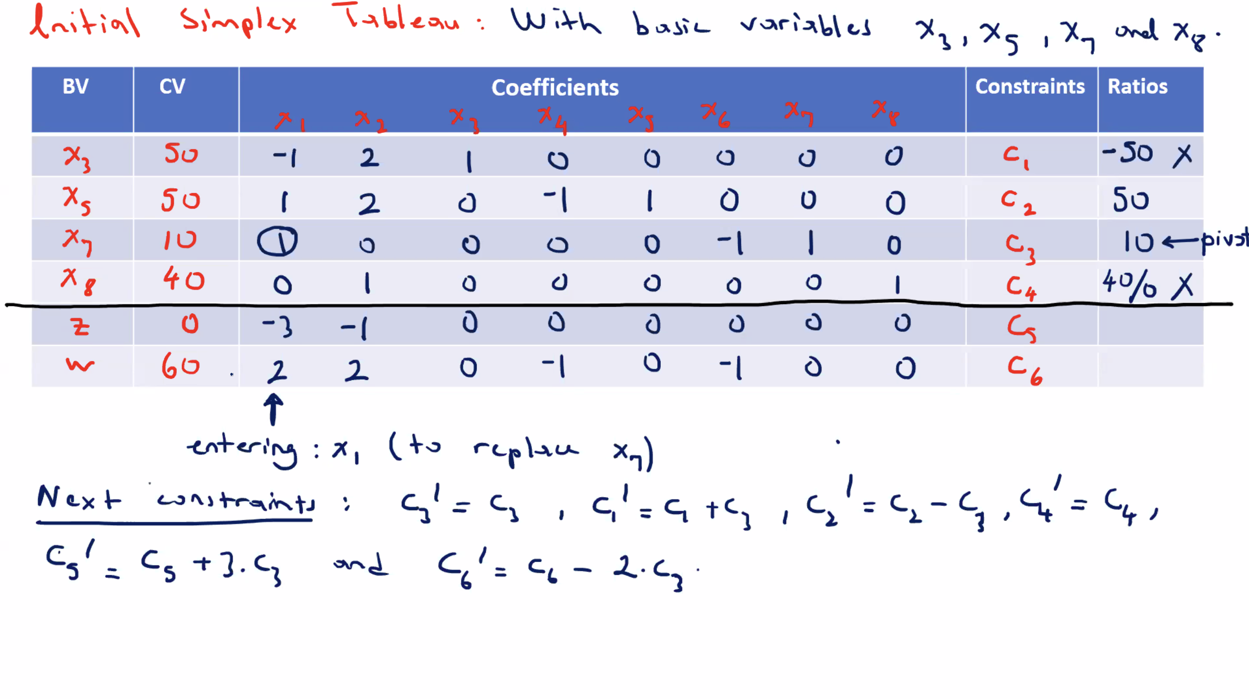
Recall previous example #

So how can we identify the shadow price when we have artificial variables by looking at the last row of the simplex tableau?

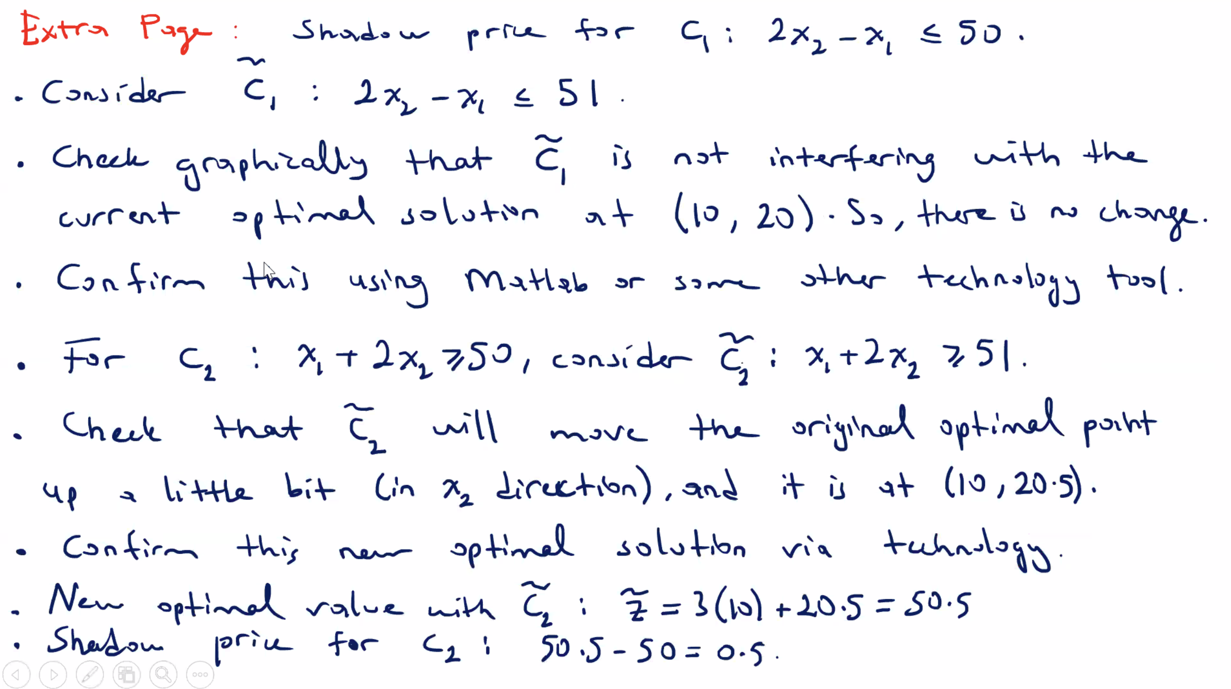
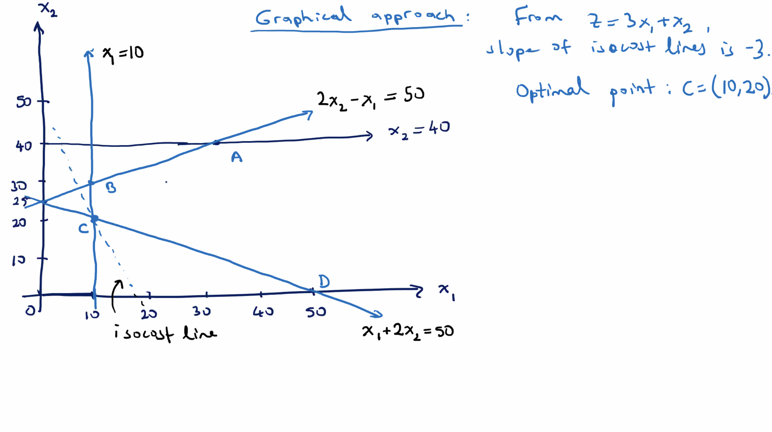
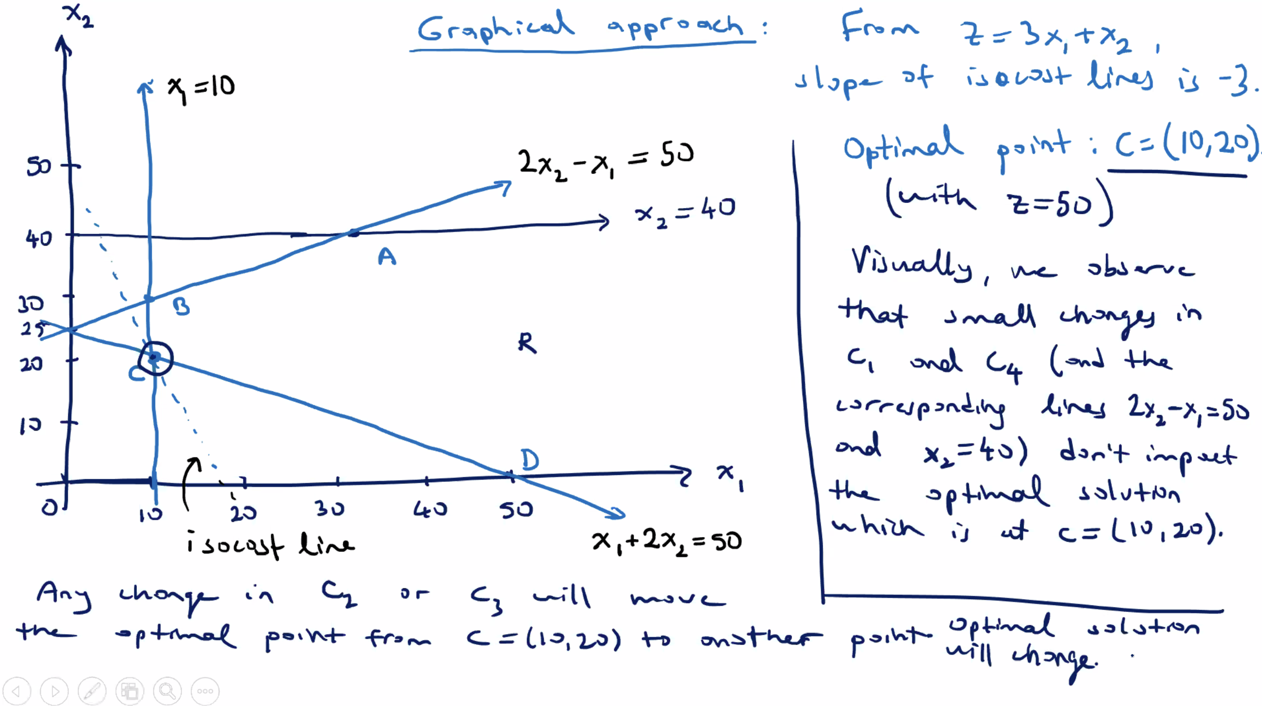
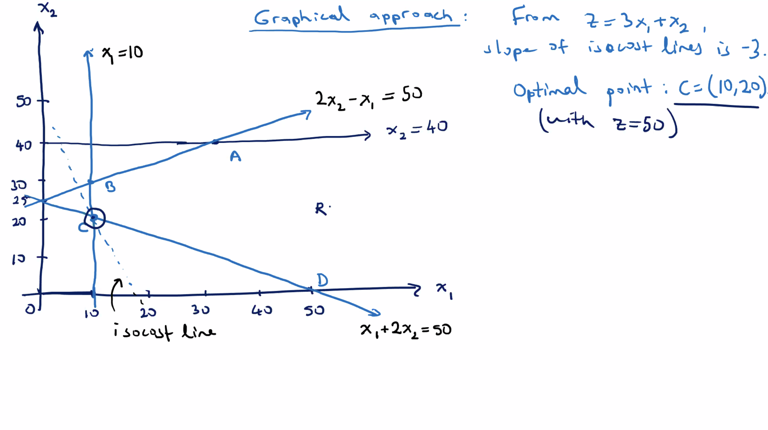
Notice that moving the upper constraint up does not change the optimal solution at point \( C \) . But if you move the lower constraint up the optimal point will change.

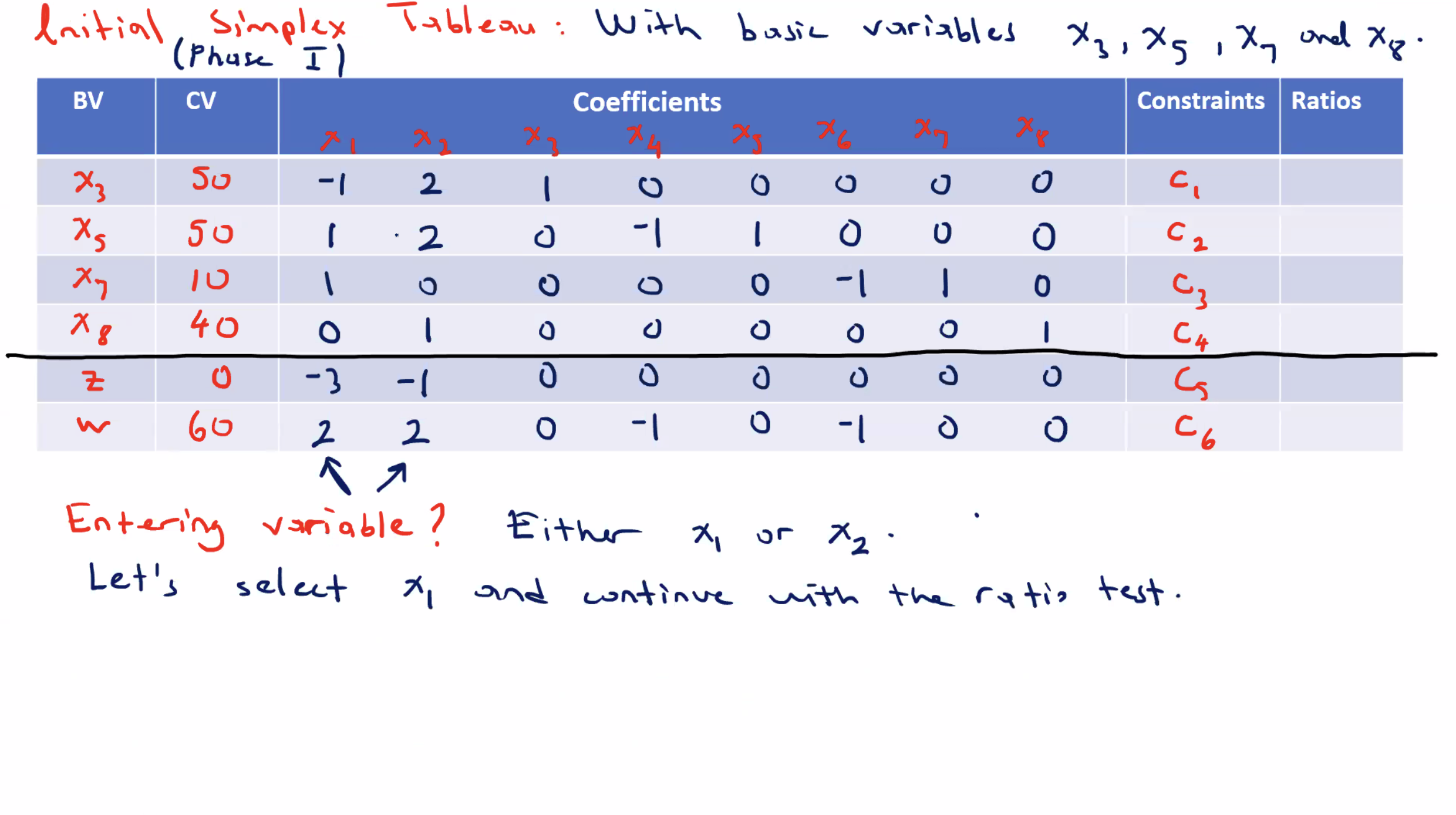
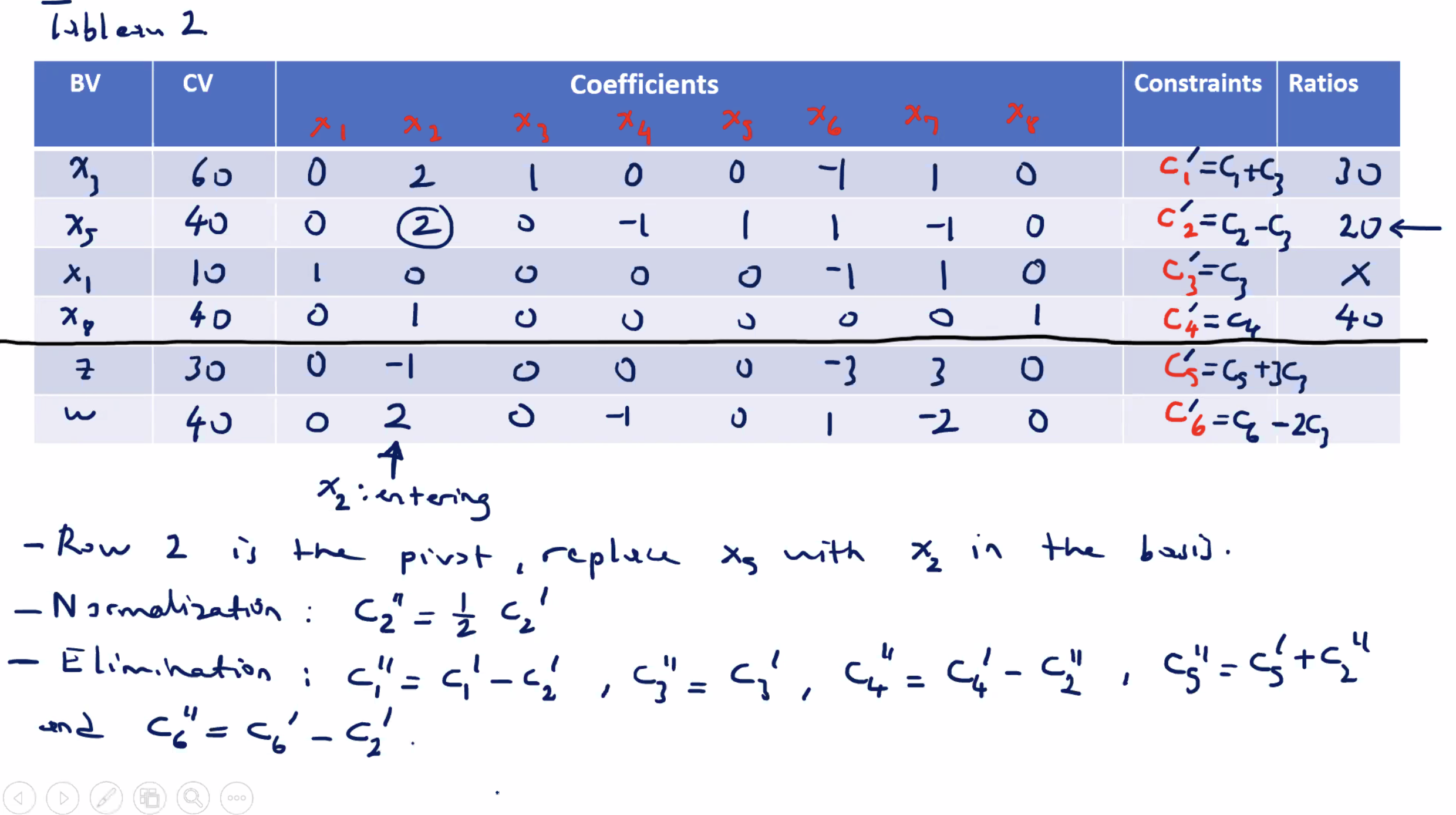
Correction: \( x_5 \) replaced \( x_2 \) , so the left hand side BV is labeled incorrect.

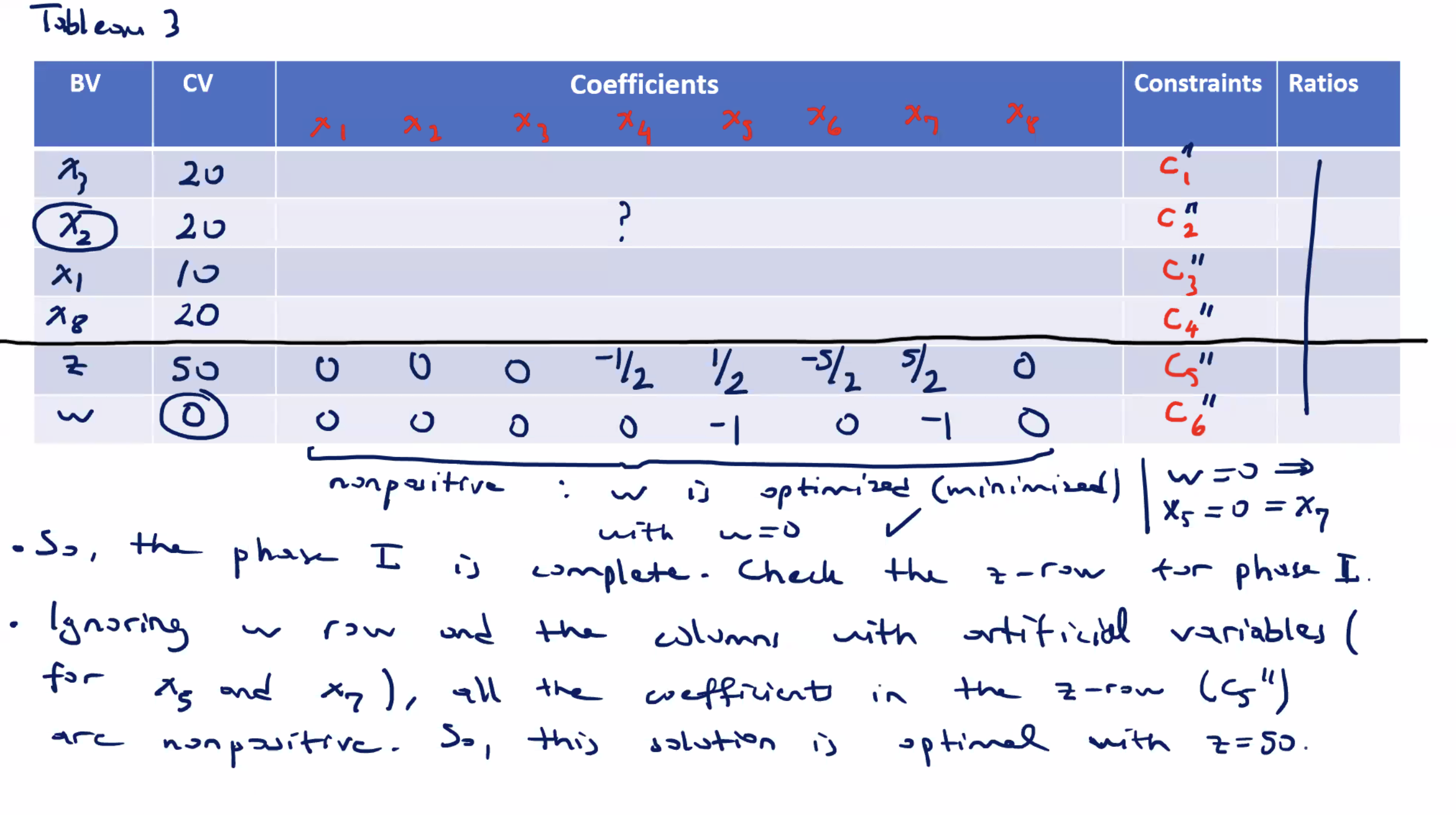
We can ignore the artificial variable columns, and still consider \( z \) optimal, because the \( w \) equation equals \( 0 \) , and \( w = x_5 + x_7 \) .

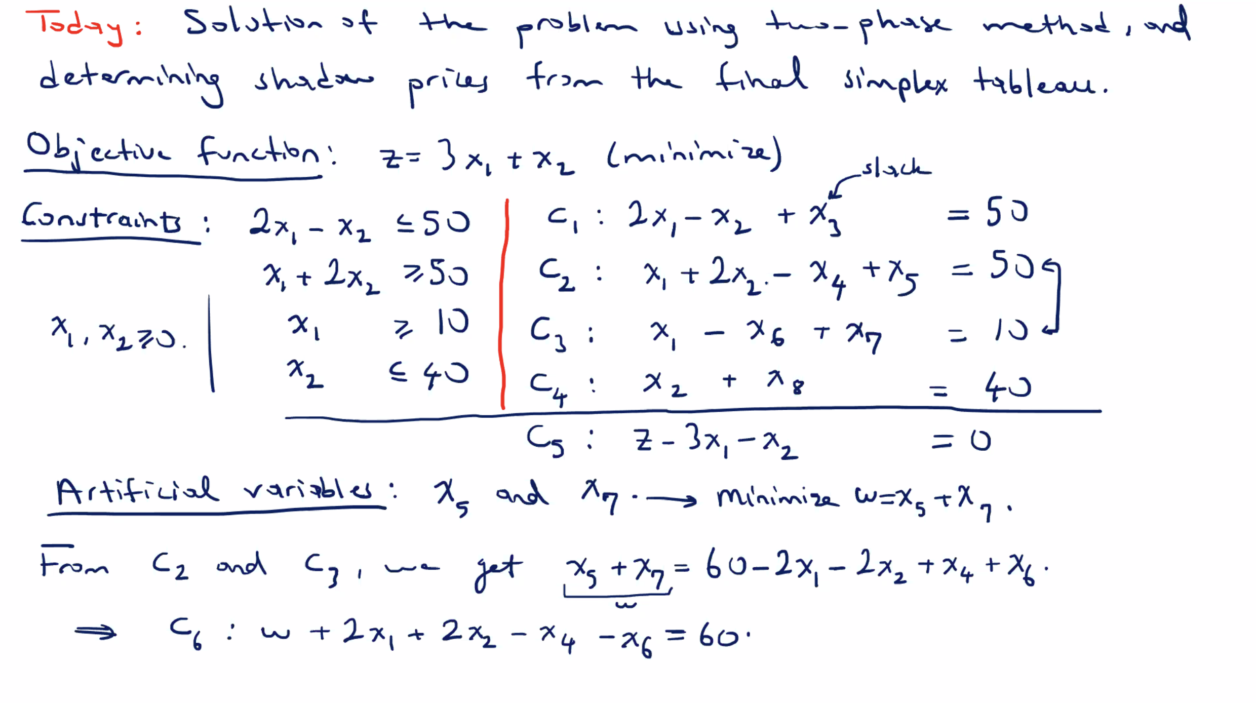
So, the optimal solution to the original minimization LP problem is \( x_1 = 10, x_2 = 20 \) with \( z = 50 \) . Now let’s check the shadow prices and how they are related to the coefficients in the last row ( \( z \) row), of the last simplex tableau.

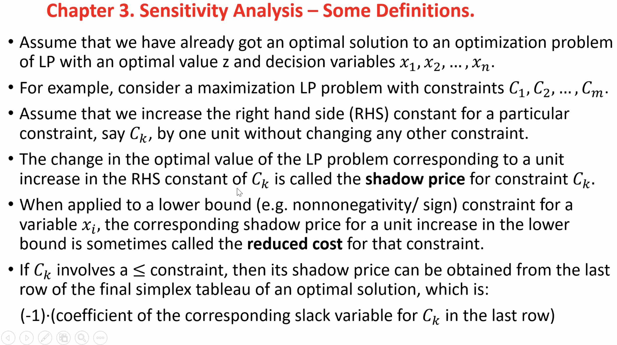
Recall,

• if it is a slack variable, we can simply multiply by \( -1 \) to obtain shadow price for corresponding constraint

Since the coefficients of \( x_3 \) and \( x_8 \) are both 0, their shadow price is 0.

Surplus variables in \( c_2 \) and \( c_3 \) : shadow price is the negative of the coefficients of the corresponding surplus variables.

• So, for \( c_2 \) the shadow price of a 1 unit increase is \( \frac{1}{2} \) . This is obtained by multiplying the slack variable \( x_4 \) by \( -1 \) .
• Similarly, for \( c_3 \) , the shadow price of a 1 unit increase is \( \frac{5}{2} \) .