Variable length encoding #

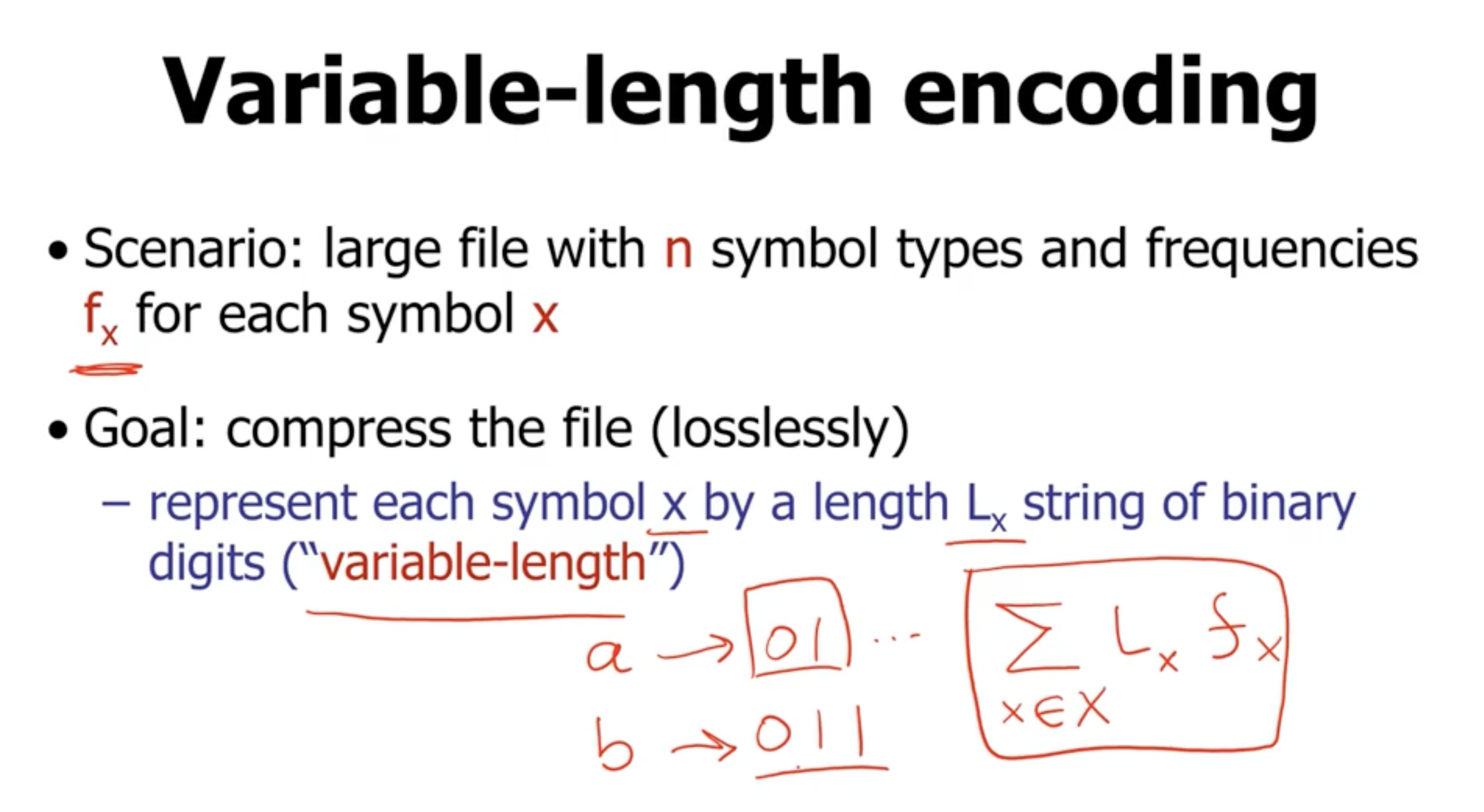
If we want to compress a file, we need to represent each symbol with a string of binary digits. If our strings are variable length, then that means the representation for any symbol should not be the prefix of the representation of another symbol.

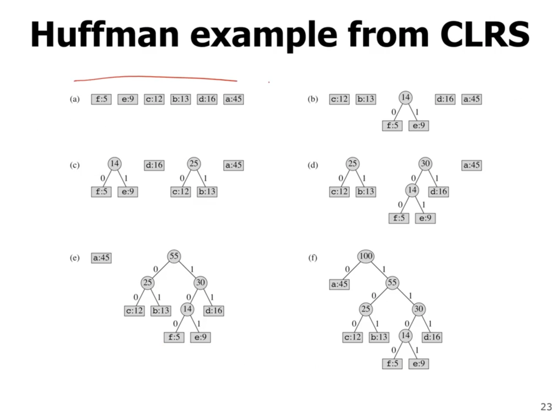
Huffman codes #

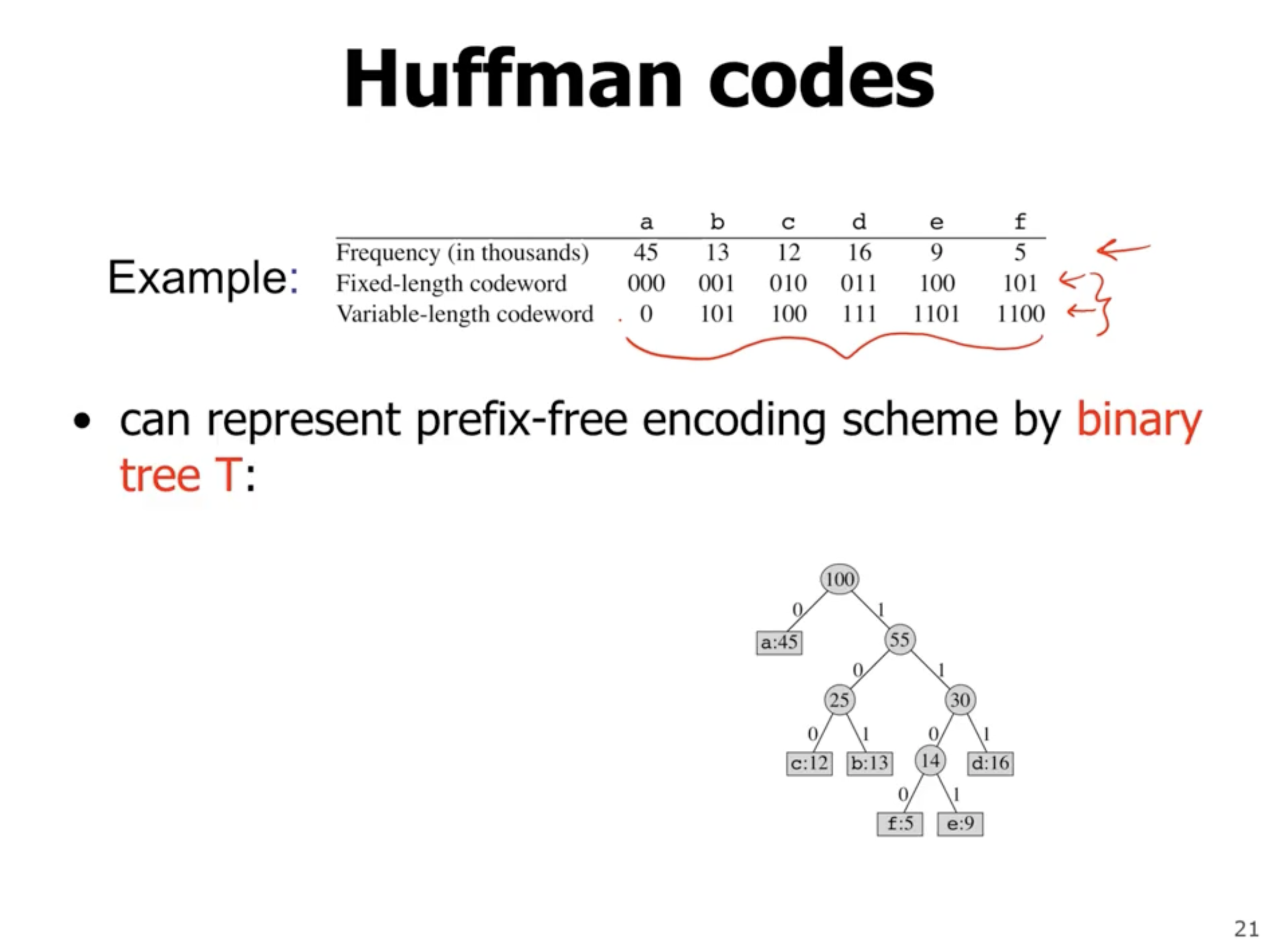
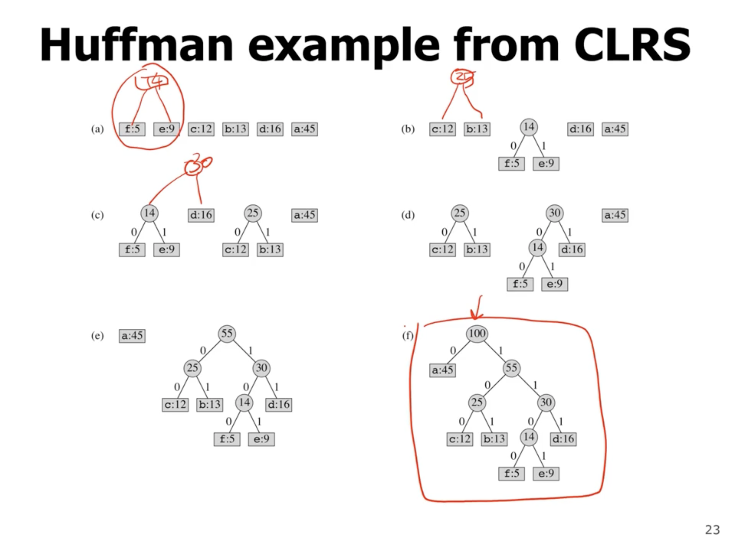
The value at each node is the frequency of symbols in the subtree. The leaves represent symbols, and each left or right child represents a 0 or 1. So, if we walk directly to a leaf, the values on each link represent the encoded symbol.

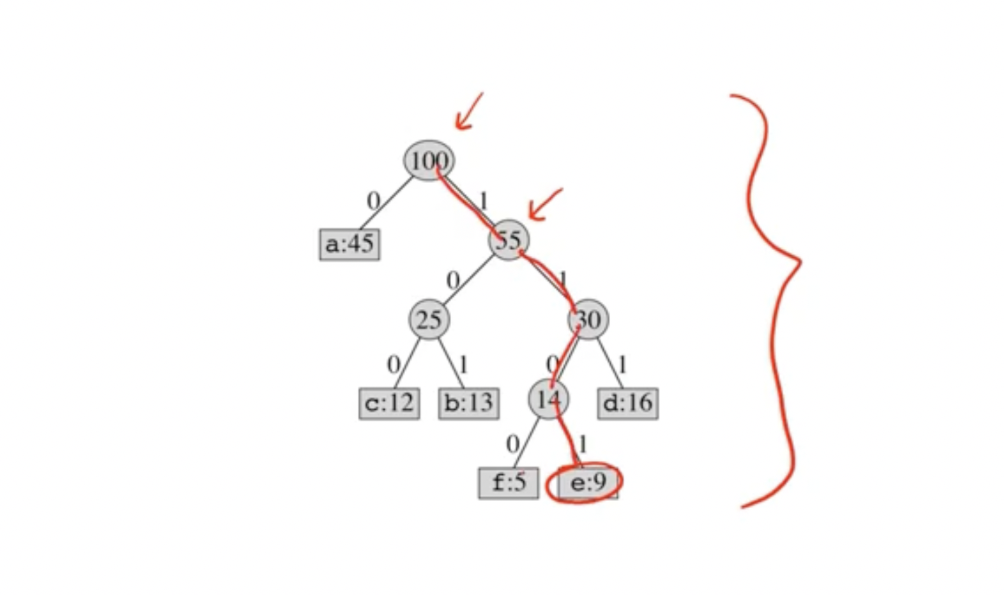
So, the above tree shows that e is represented as 1101.

So how can we optimize this tree using a greedy algorithm? First off, we want the lowest frequency symbols to as low as possible in the tree (lowest frequency items have longer encodings).

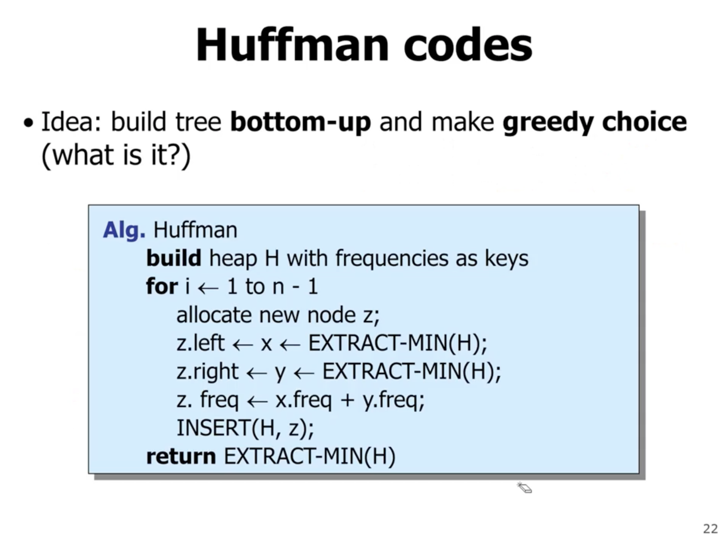
• \( n \) is the number of symbols
• creates a heap with frequencies
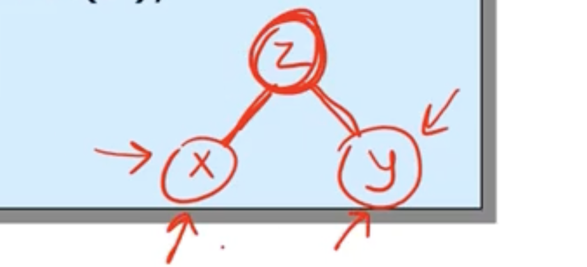
• each iteration extracts 2 nodes from heap, and inserts a new node that has the sum of frequencies

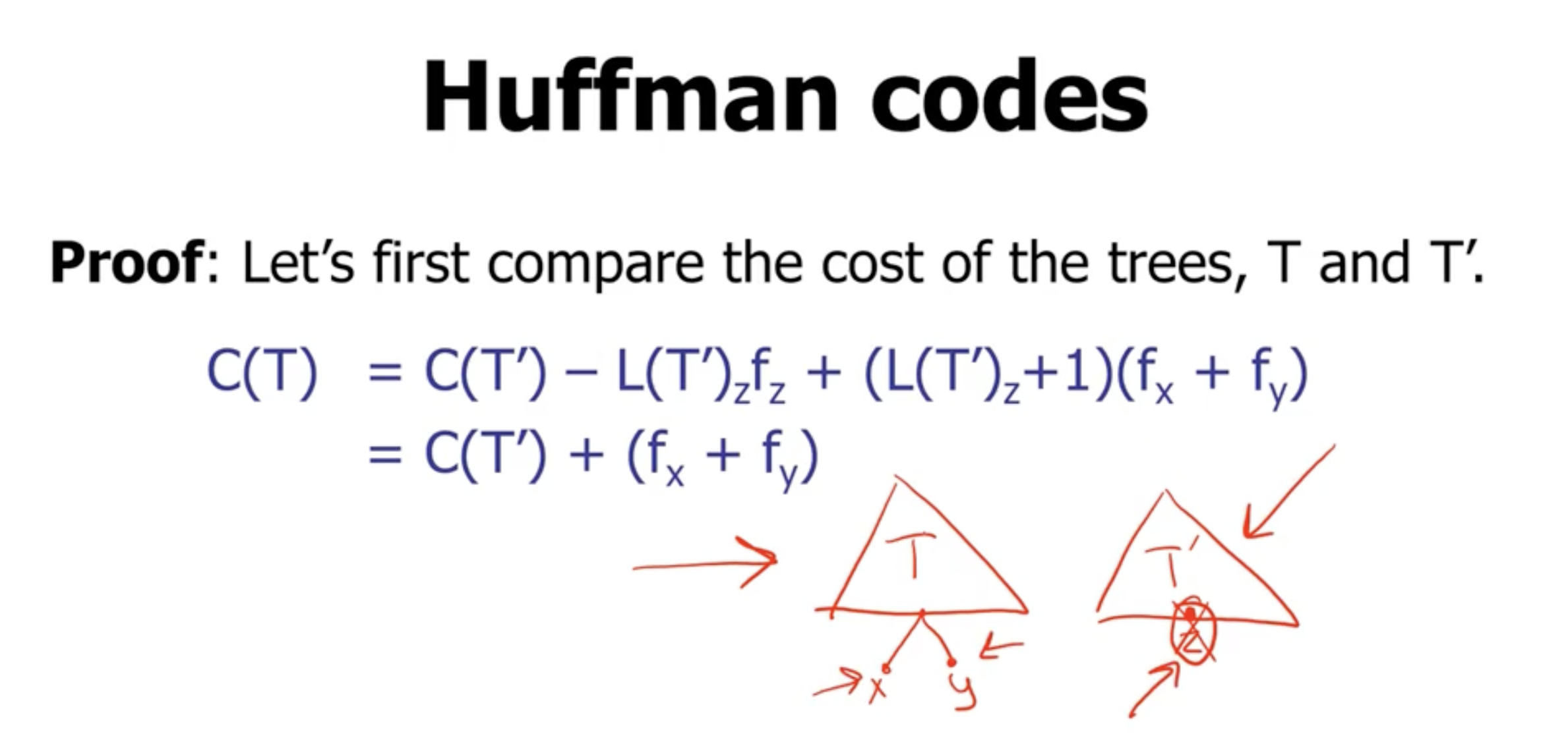
So how do we prove that this is the optimal binary tree? We need to prove

• the greedy choice property
• the optimal substructure property

At each point, we are always choosing the 2 lowest frequency symbols.

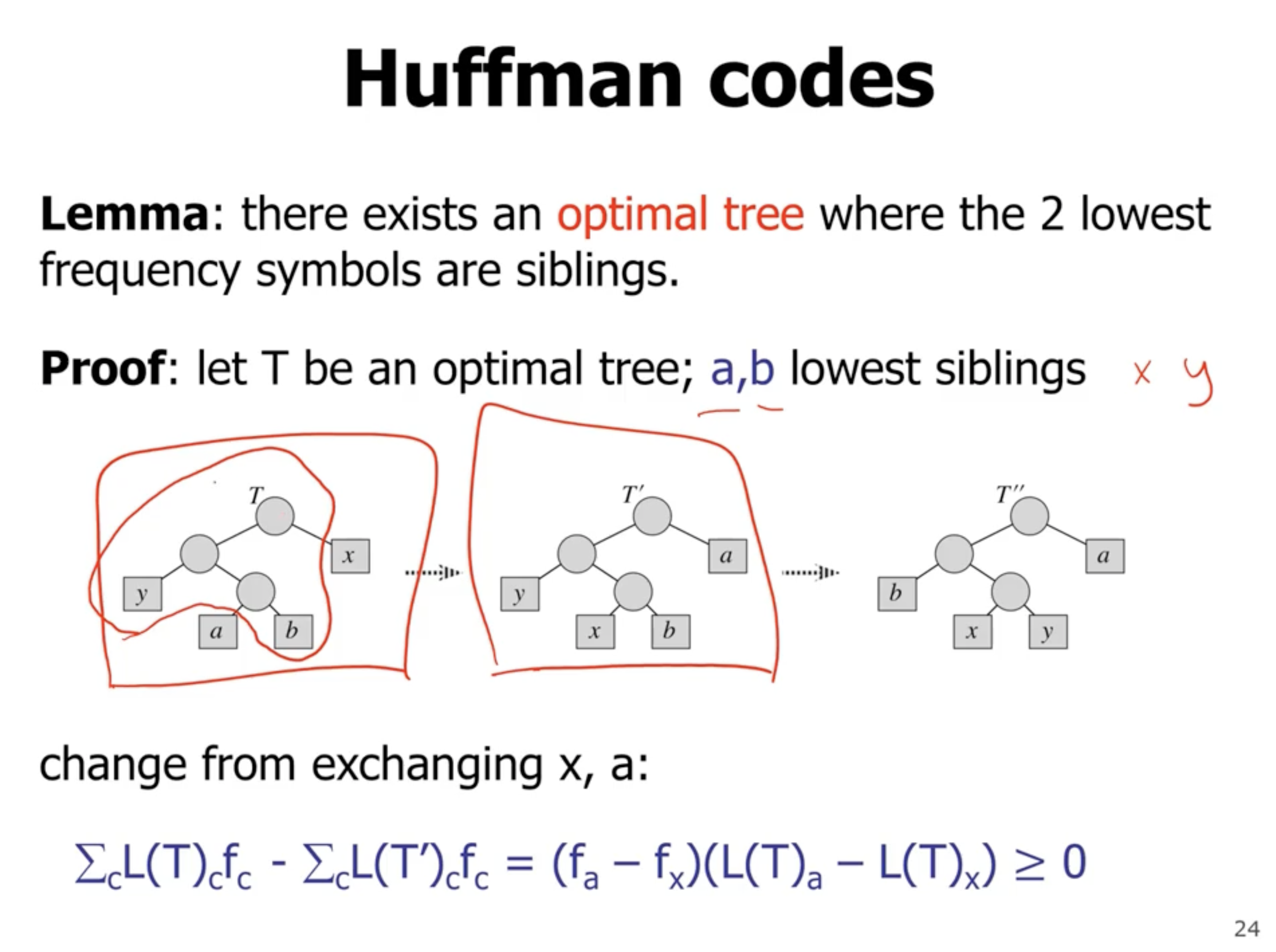
If during each swap, the subtree frequency does not change, then each tree is optimal.

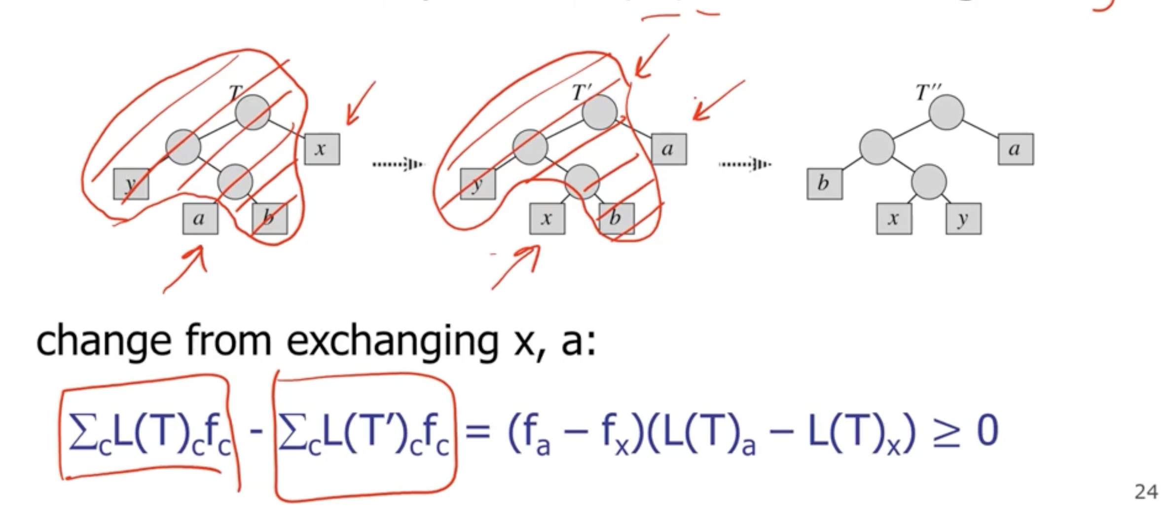
The reason that it is \( \geq 0 \) is because it will have either lower or the same frequency.

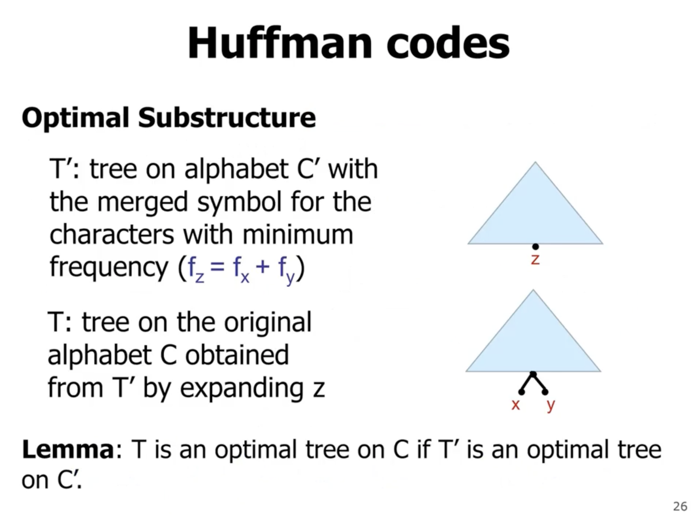
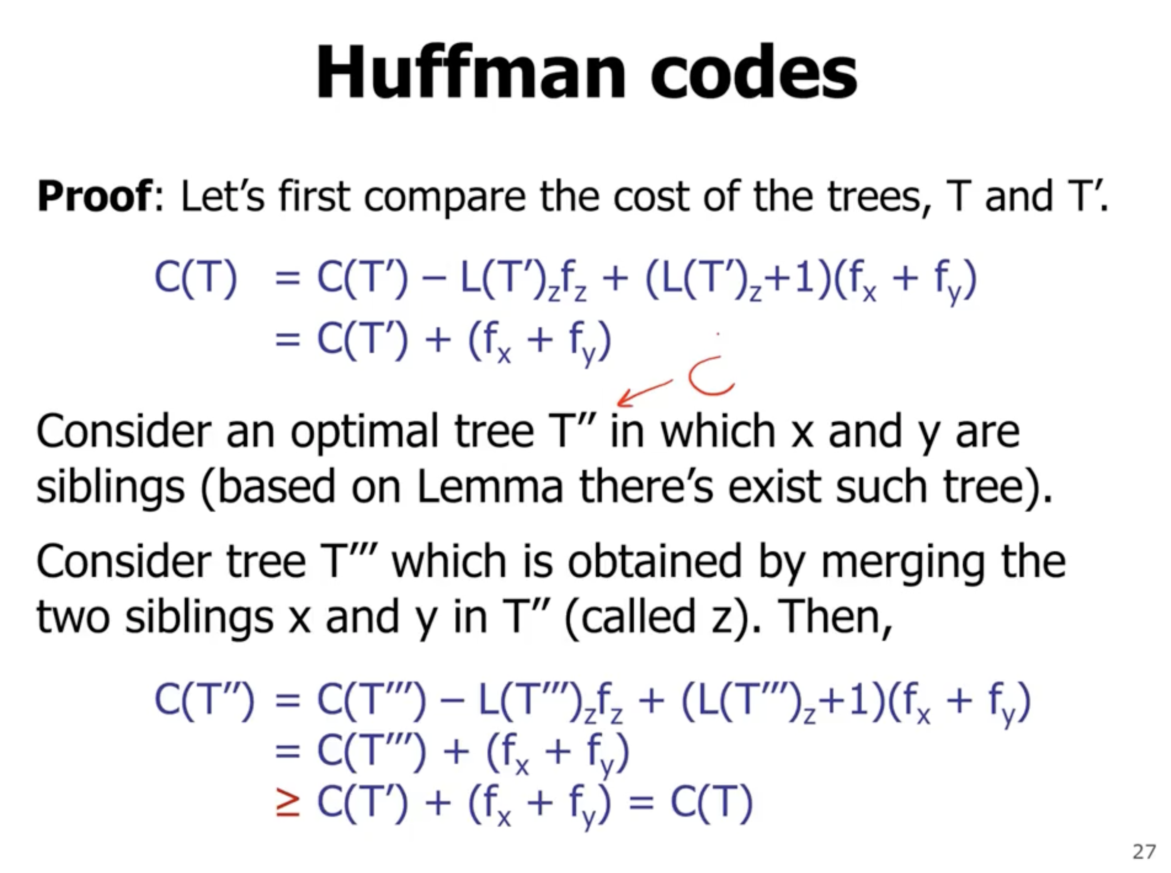
Based on our assumption, we think that \( T' \) is optimal, whereas \( T''' \) may not be optimal. That is why the cost of \( T'' \) is \( \geq \) to \( C(T) \) .

Minimum spanning trees #

Finding a minimum spanning tree in a graph is also a greedy algorithm.

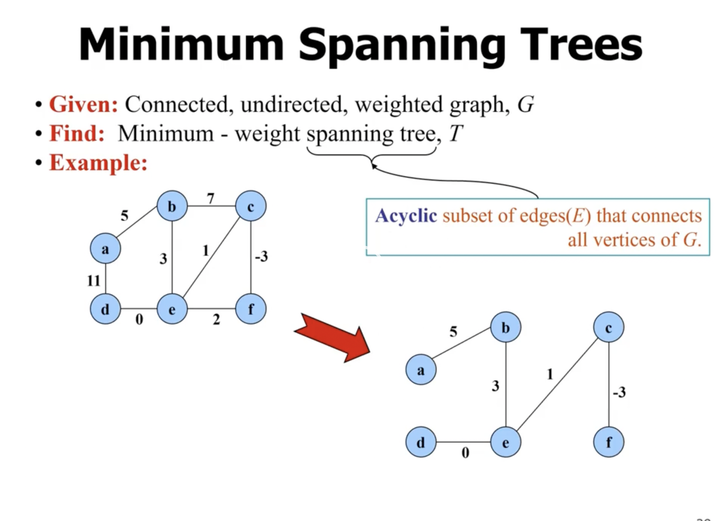
• spanning means it covers every node in the graph
• tree means there is no cycles
• minimum means that the total cost of the tree is the lowest possible

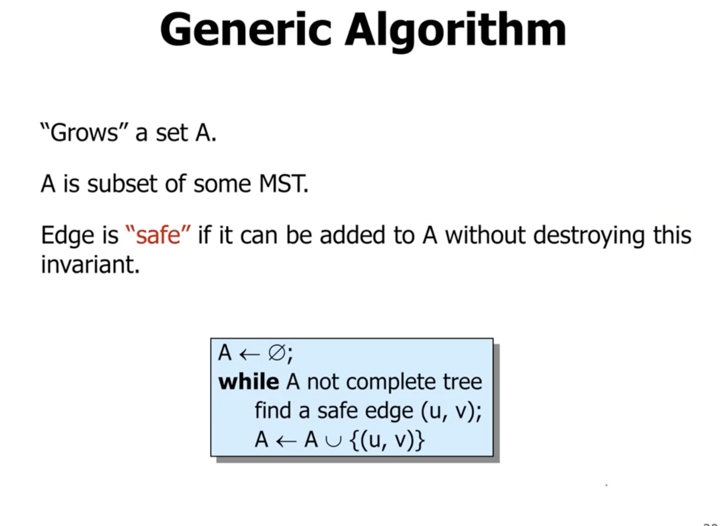
• “safe” means that when adding an edge to \( A \) , it is still a subset of the MST

So how do we find the safe edge? That leads to different algorithms.

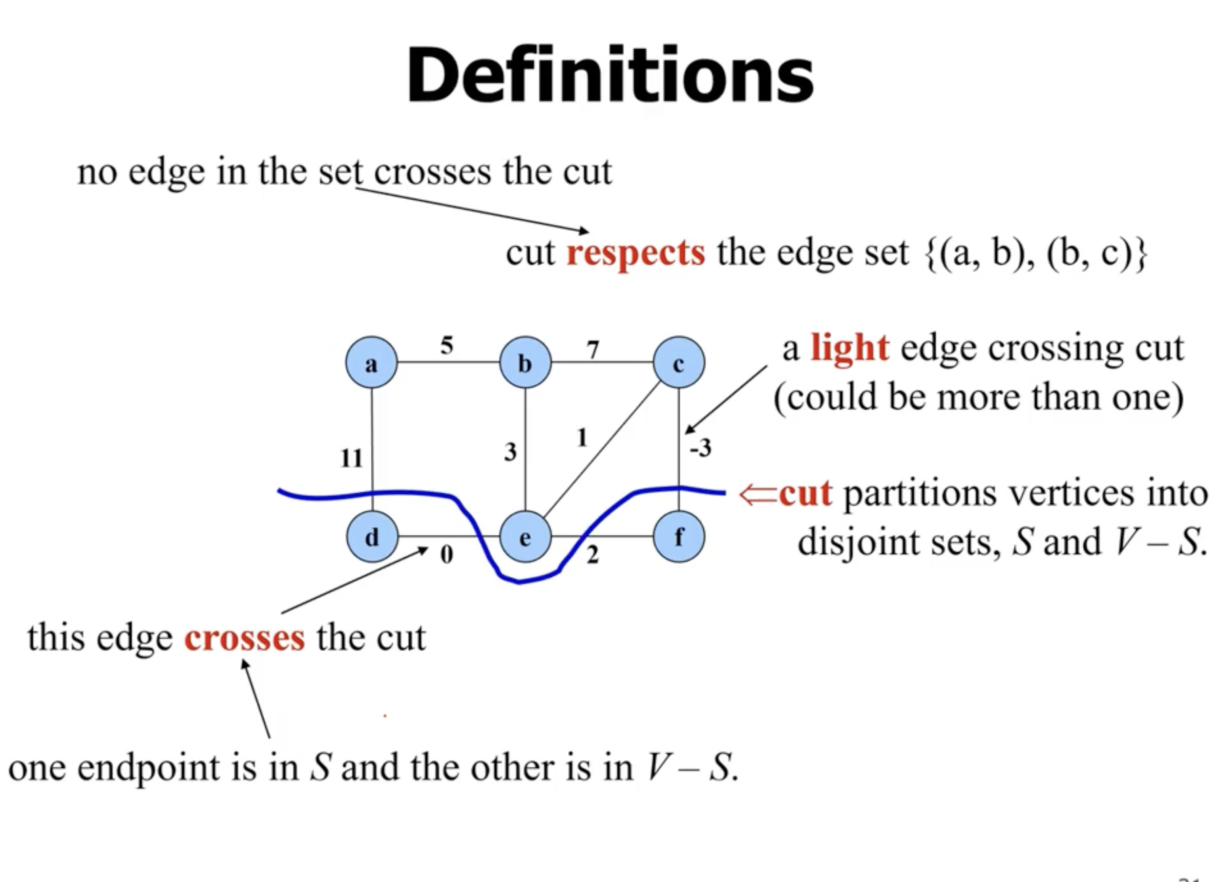
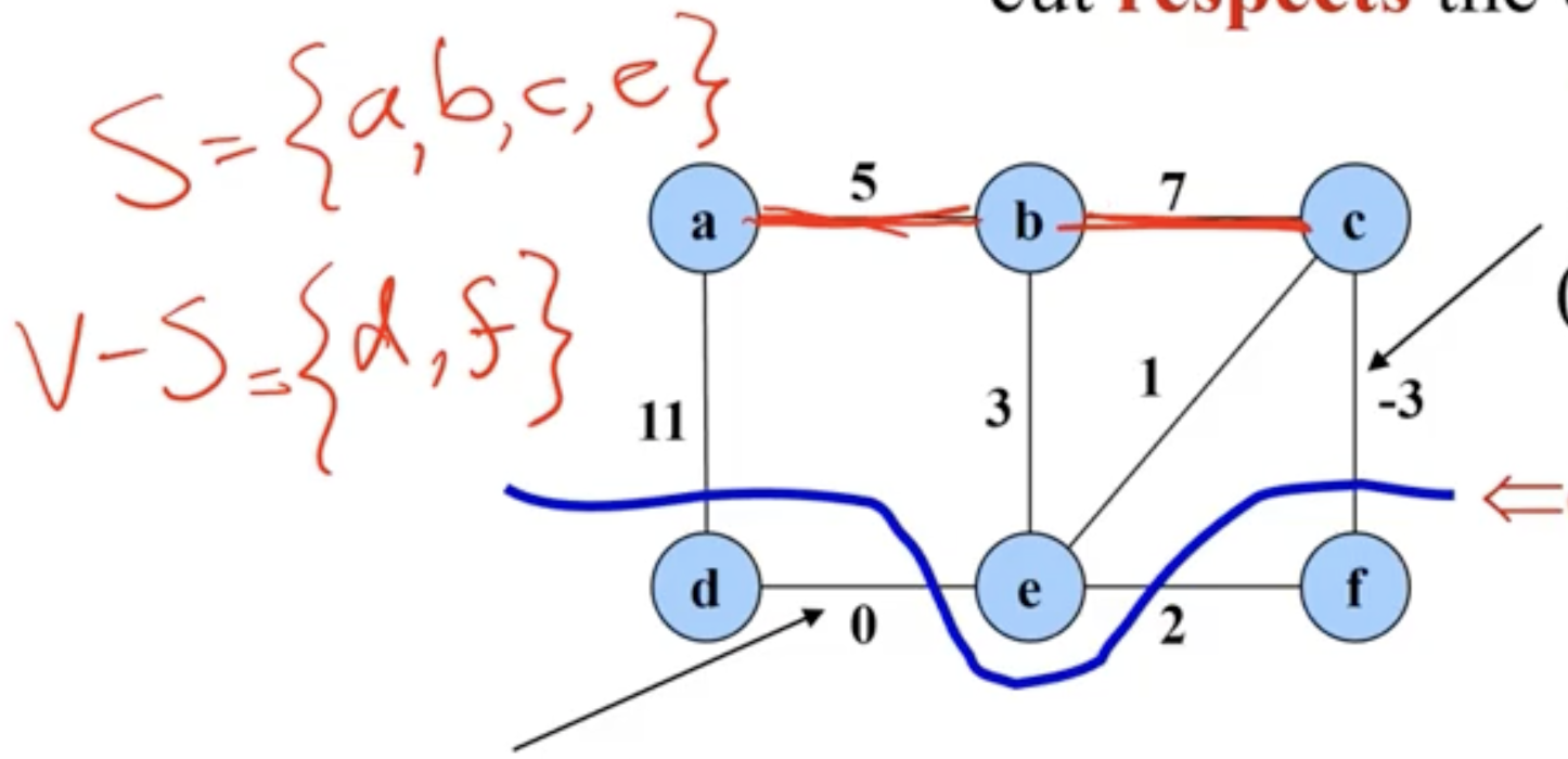
• an edge that “crosses the cut”, means it has 1 endpoint in the first set, and 1 endpoint in the other.

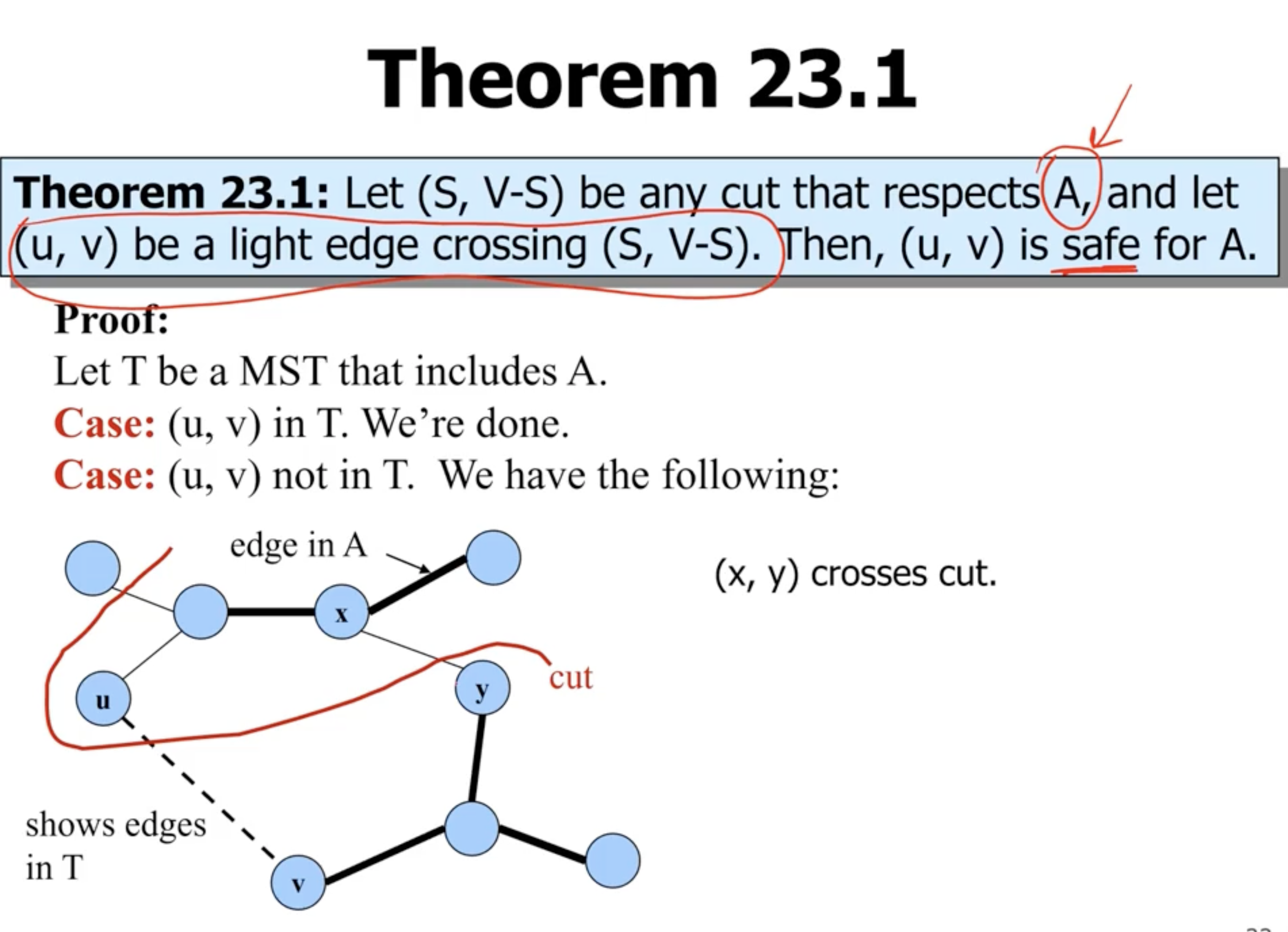
• there should be at least 1 edge that crosse the cut, for example \( (x,y) \) .
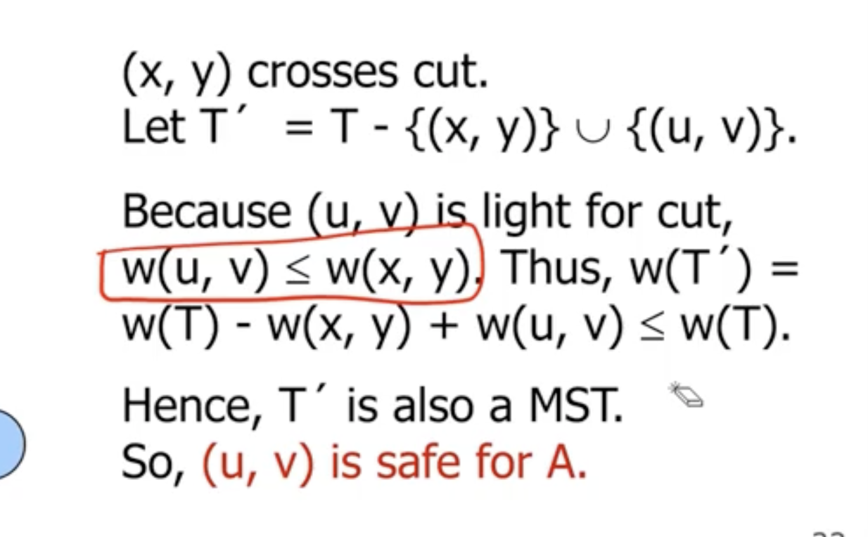
• if we remove that edge, and instead add the light edge \( (u,v) \) , that means that it is the smallest edge that crosses the cut
• this leaves us with another tree, with a total weight that is the same minus \( w(x,y) + w(u,v) \)

• “CC” = connected component

MST algorithms #

• the algorithm starts by assuming all nodes in the graph are individual connected components (nothing is connected to each other, no nodes in the MST yet)

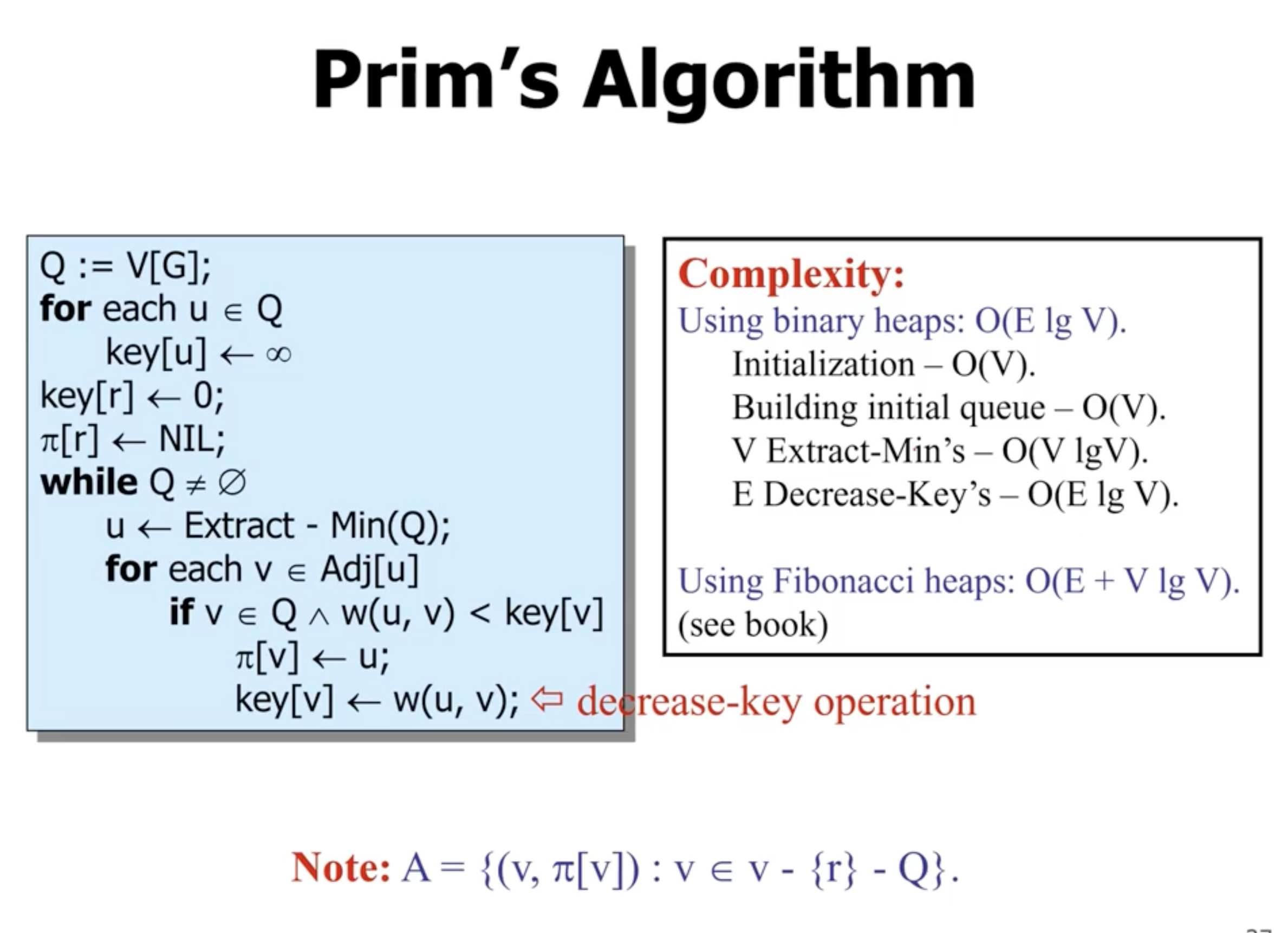
• \( \pi[r] \) represents the “parent of node \( r \) ”
• extract-min in a binary heap has a runtime of \( O(\lg n) \)
• decrease-key operation has a complexity of \( O(\lg V) \)
• the amount of edges in a connected graph is \( E = V-1 \) , or \( \Omega(V) \)
• overall runtime complexity of Prim’s is \( O(E \lg V) \)

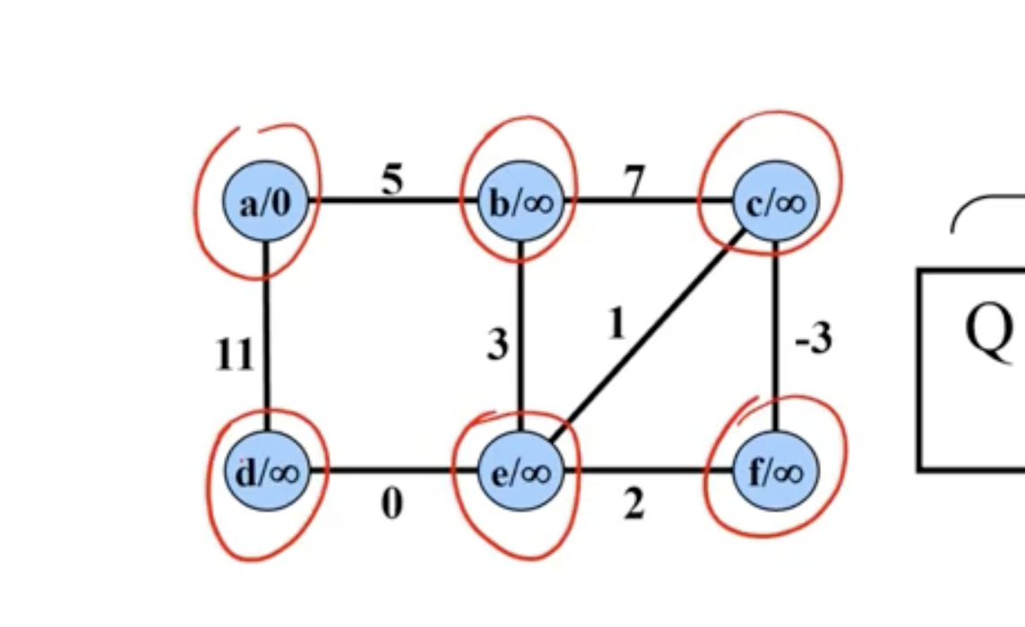
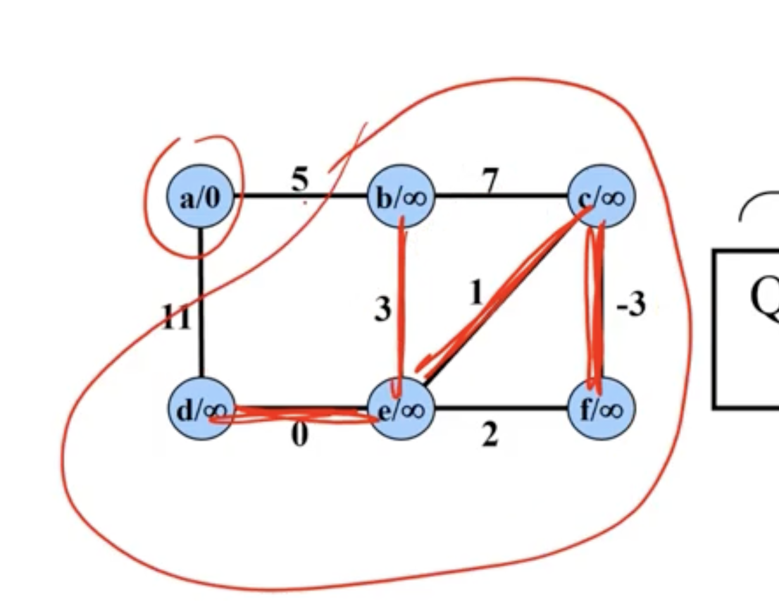
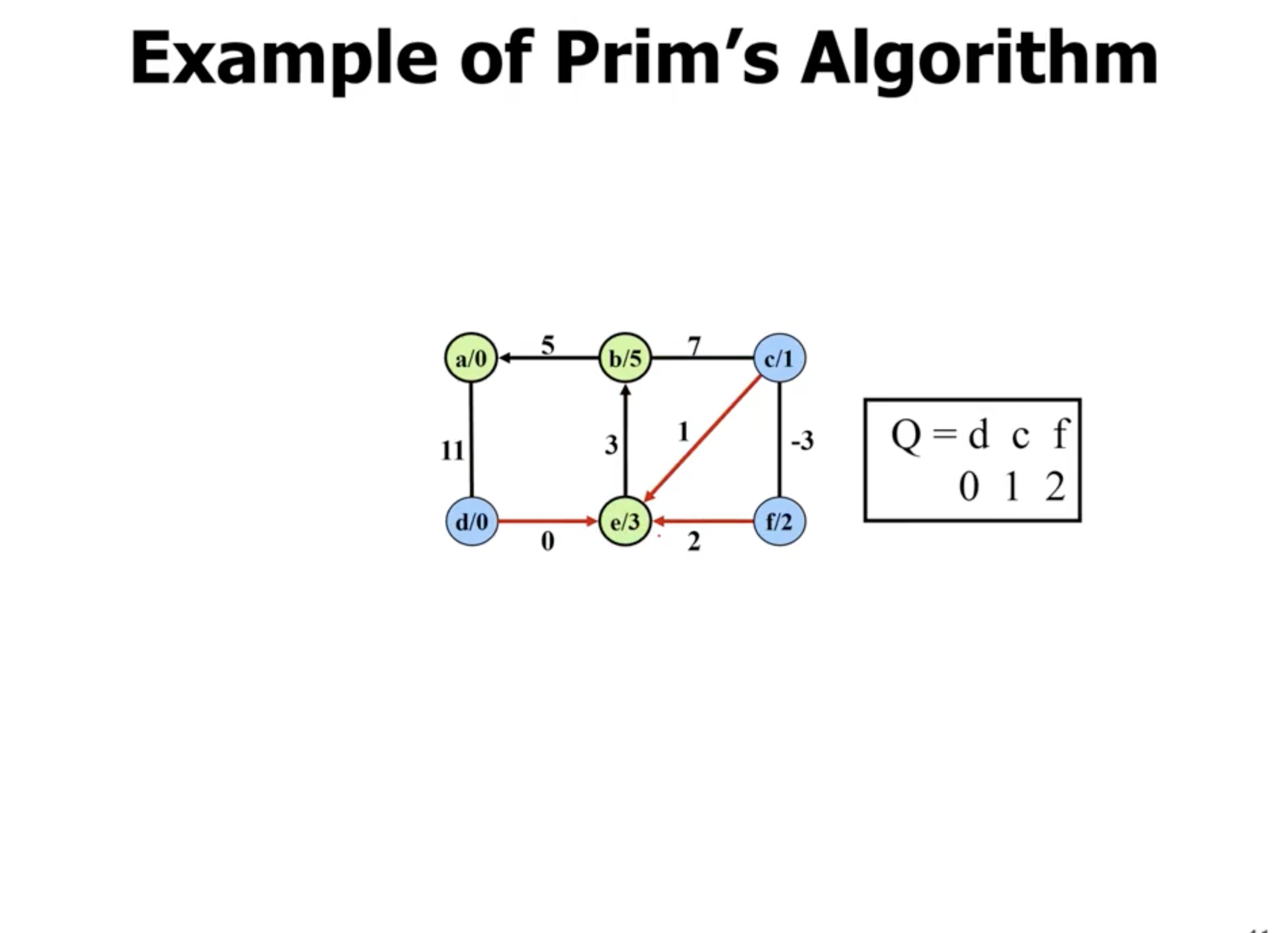
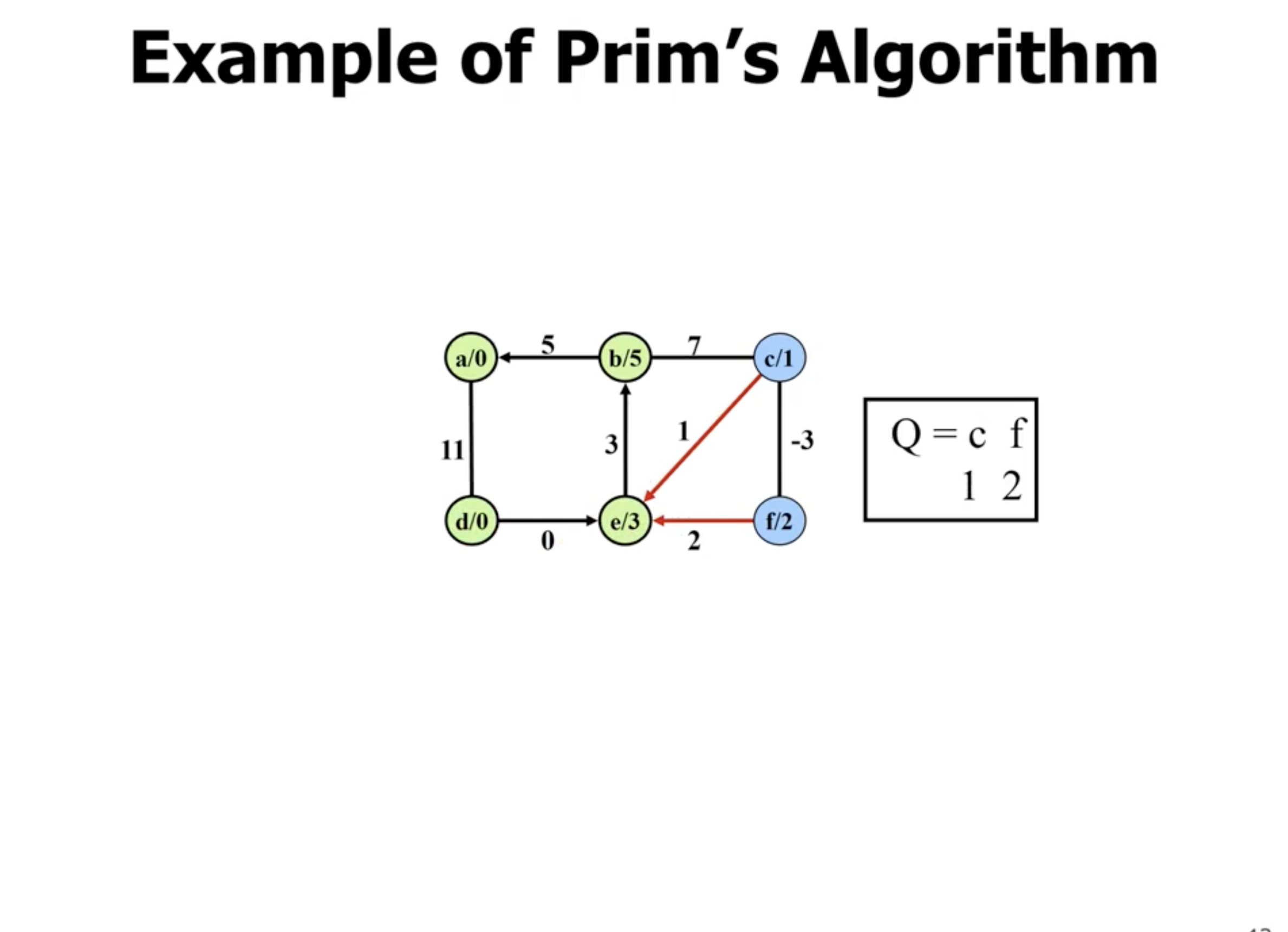
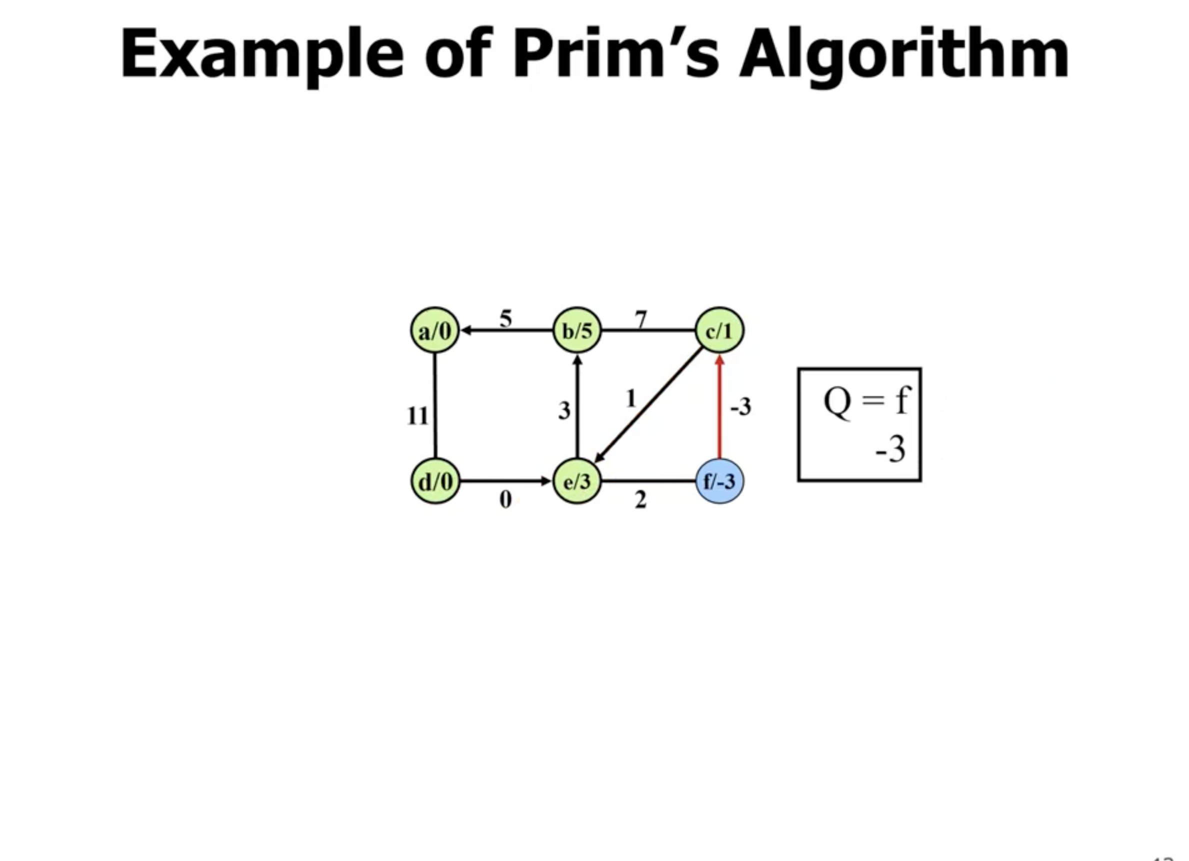
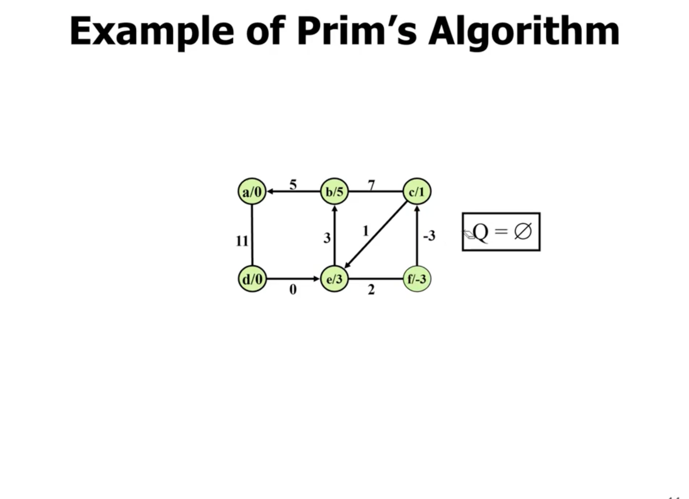
Example of Prim’s #

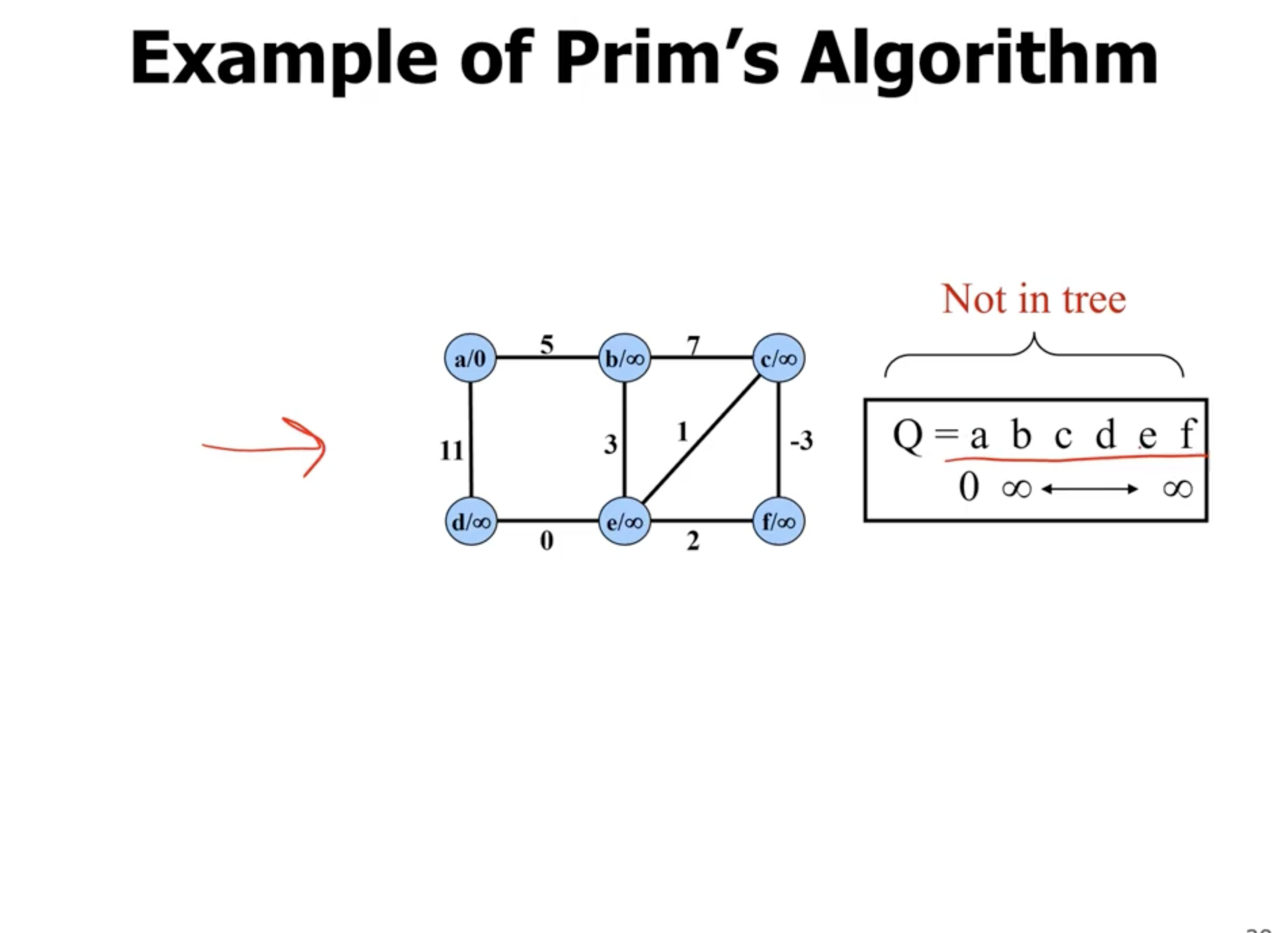
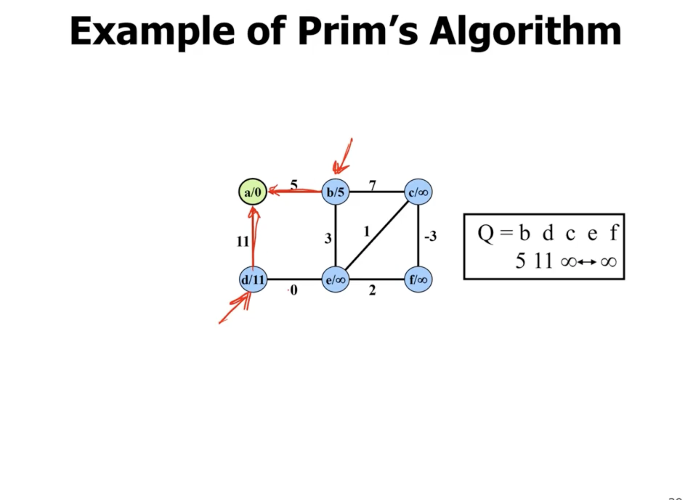
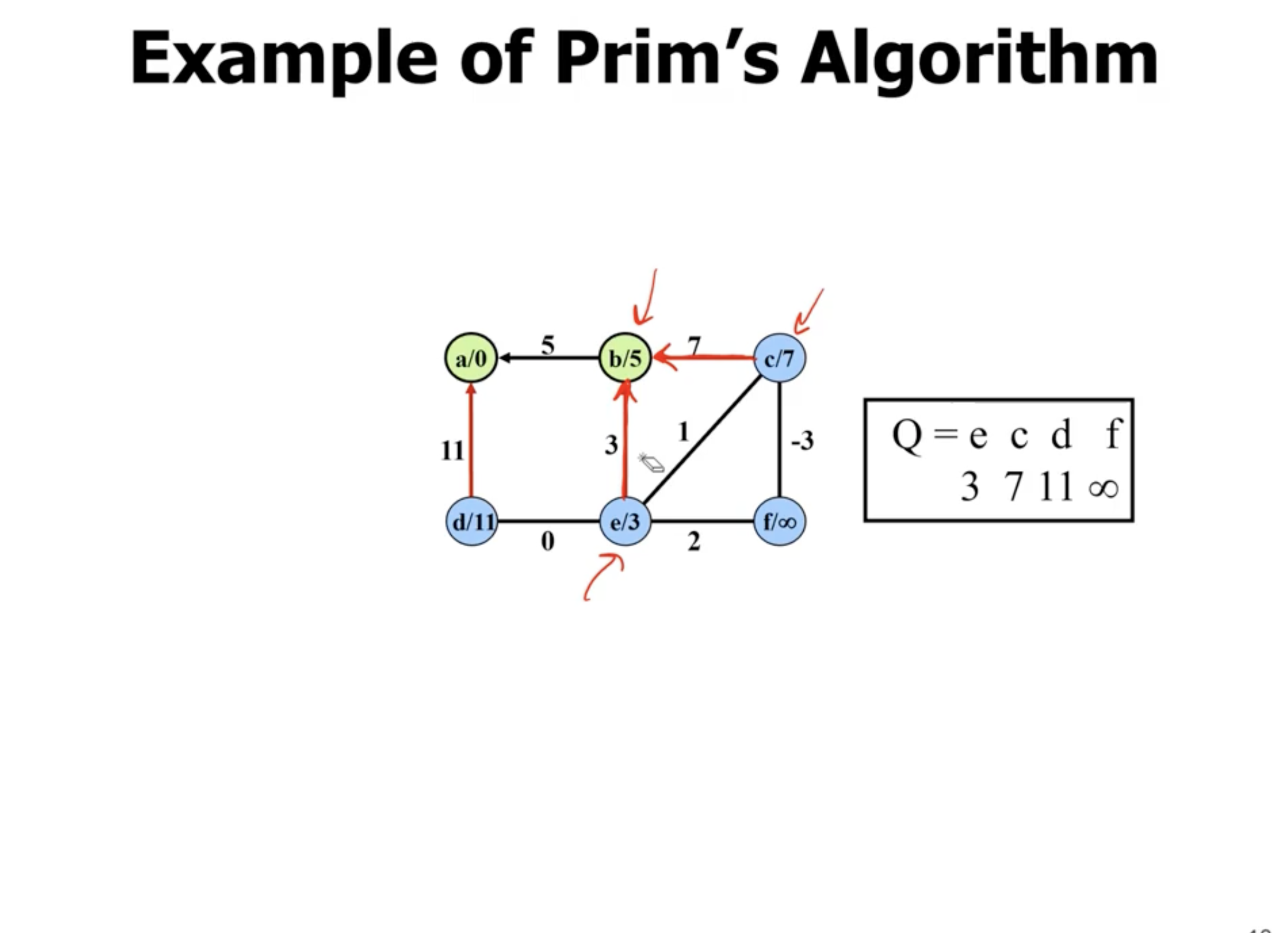
Note: This is not a directed graph, the arrows just show what nodes are directly being updated when a new node is added.

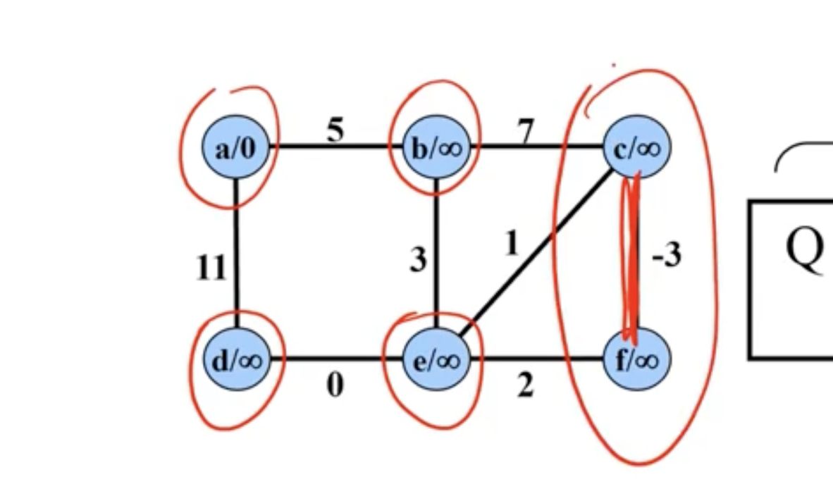
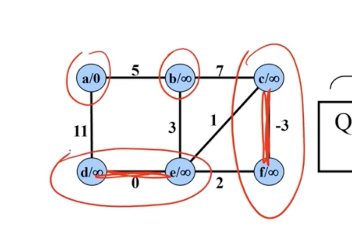
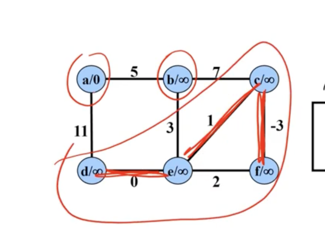
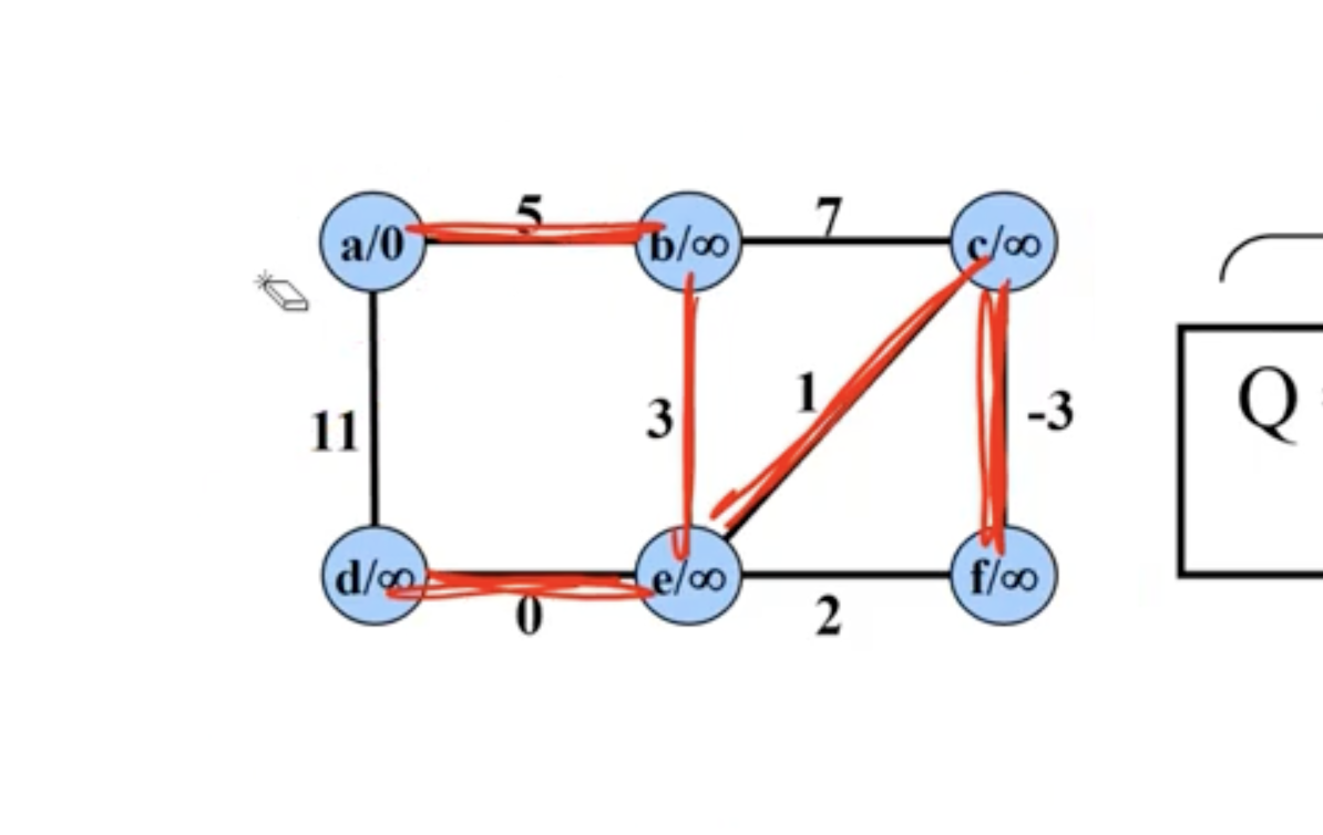
Example of Kruskal’s #

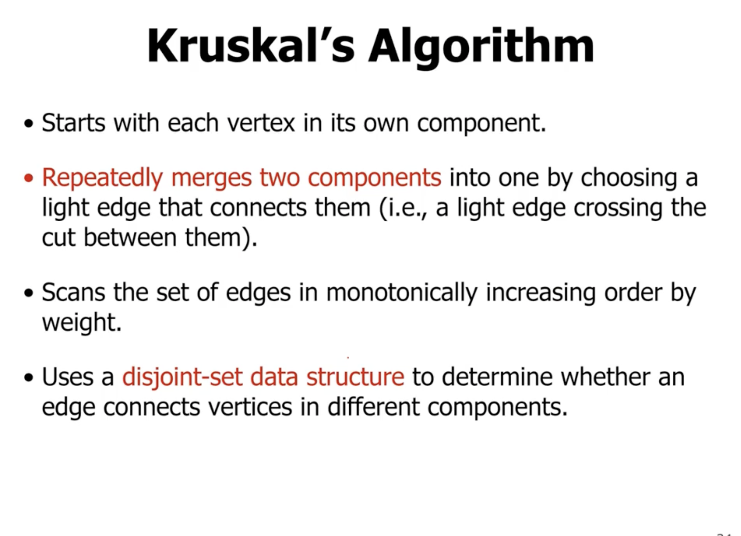
In comparison, Kruskal’s starts with all nodes being their own connected components. It chooses the minimum edge between any 2 connected components:

Note: Disregard the \( \infty \) signs in each node here, we're just reusing the graph from the Prim's example to show Kruskal's.