Cryptographic hash functions #

Hashing takes a very large domain and maps it to a smaller codomain. For this to scale nicely,

• the hash function must be fast
• the outputs must be fairly random in distribution

A hash function can be defined as \( H : \{0,1\}^* \to \{0,1\}^b \) , where \( b \) is the output block length.

Recall: a set raised to an asterisk means the set of all strings made from that set.

We insist a cryptographic hash function has these properties:

• Preimage resistance: it should be non invertible. If we know an output, we shouldn’t be able to find an input that produces that output. Given \( y \) , it is hard to find any \( x \) such such that \( H(x) = y \) . This should just be really hard to find (near impossible). Note that since we have an infinite input, there definitely are multiple values that map to the same output value, but it should be near impossible to find them.
• Second preimage resistance: if we have another value, it should be hard to find another value that map to the same output. Given \( x_1 \) , it is hard to find \( x_2 \neq x_1 \) such that \( H(x_1) = H(x_2) \)
• Collision resistance: it is hard to find any pair that cause the same output. It is hard to find \( x_2 \neq x_1 \) such that \( H(x_1) = H(x_2) \)
• A nice to have property: behave like a public random function (random oracle).

Since hash algorithms aren’t invertible, they are useful for

• fingerprints
• message authenticity, if two the sender’s and receiver’s copy of the message being sent both hash to the same value, it can be considered authentic
• some file systems use hash functions to determine if a file has been changed

Some history for hash functions #

MD5

• Invented in the 90s
• block size of \( b = 128 \) bits
• MD5 is now broken, as pairs of input which produce the same output can be found rather easily now.

SHA-1

• Invented in the 90s
• block size of \( b = 160 \) bits
• broken, deprecated

SHA-2

• a fixed version of SHA-1, considered secure
• also called SHA-256, SHA-512
• block size can be \( b = 256 \) or \( 512 \) , respectively.

SHA-3

• competition to find next best hash algorithm
• Same style contest as AES, winner was Keccak
• block size \( b = 256 \) or \( 512 \)
• considered secure

Telephone coin flipping #

Imagine a friend flipping a coin on the other end of a phone call. Your friend may think that you may cheat and have no way of knowing. In fact, you could cheat and your friend wouldn’t know.

How could they use a hash function to ensure no one is lying?

• let person \( A \) pick a random \( x \) , 128 bits
• \( A \) tells \( B \) the hash value \( H(x) \)
• \( B \) chooses 0 or 1, and tells \( A \)
• \( A \) tells \( B \) the value \( x \)
• consider the last bit of \( x \) to be the answer to the coin flip, \( 0 \) = heads and \( 1 \) = tails.
• \( B \) wins if last bit of \( x \) matches guess

By sending \( H(x) \) , \( A \) is commiting to the input \( x \) . It is hard for \( B \) to find the input \( x \) when they only know the hash value \( H(x) \) , so it is hard for \( A \) or \( B \) to cheat.

Hash constructions #

Recall the signature of a cryptographic hash function,

where \( b \) is the block size.

Merkle–Damgård construction #

Merkle–Damgård wikipedia

Since this function doesn’t take any key, you just feed it data and it returns the result of the hash function.

There are some initial constants that are concatenated with a chunk of the input, and that is fed into a compression function.

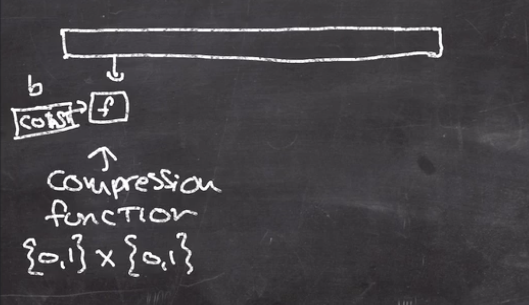
The output of this function is fed into the next compression function,

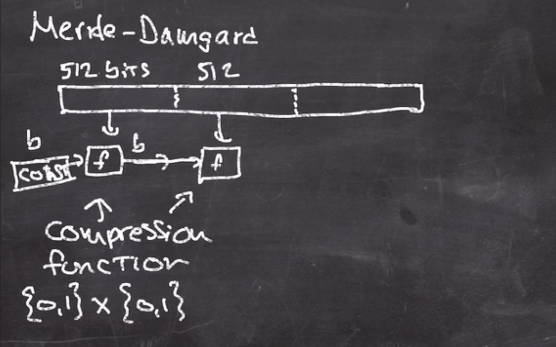
The last block must be padded to a multiple of the block size, in this case \( b = 512 \) . We will use our 10* padding algorithm for the last block - 64 bits. The length is concatenated onto the end

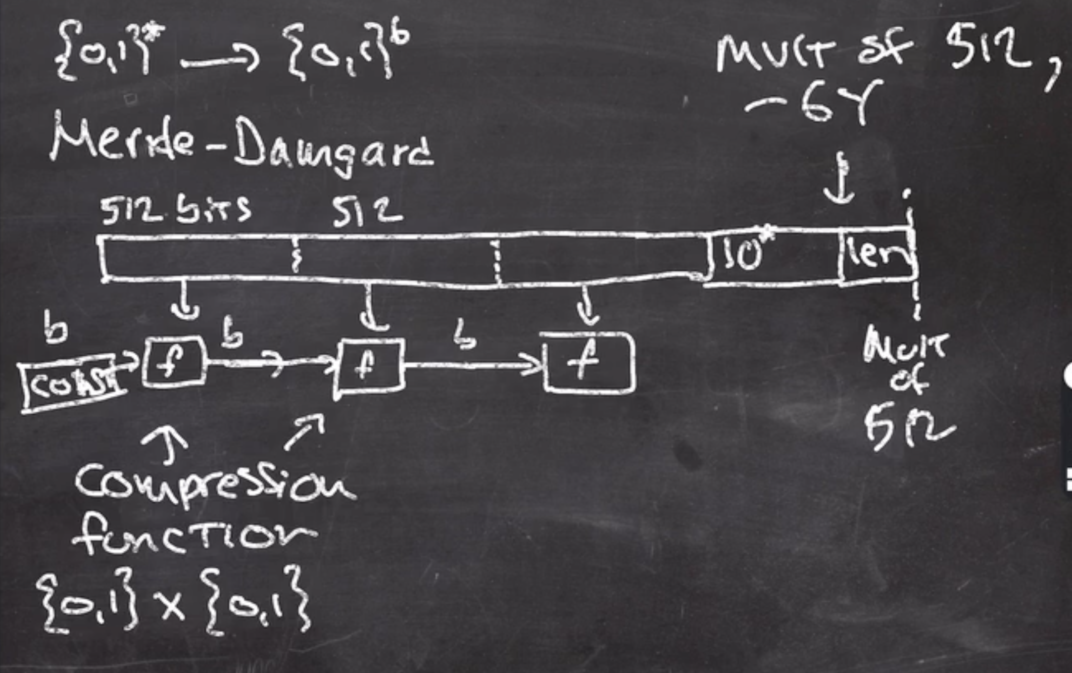
The output of the last call to the compression function \( f \) is the hash output, and we can think of \( f \) as a public random function.

So, \( f \) should be

• collision resistant
• preimage/second preimage resistant

Compression functions like \( f \) usually have

• lots of rounds
• mostly bitwise operation

Read more about the compression function in SHA-1 here.

MD5, SHA-1,2 use this same basic construction. Since these hash functions are considered broken.

Also, since the output is the last call to the hash function, it opens up the function to length extension attacks.

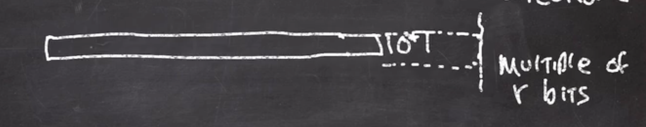
Keccak (SHA-3) – sponge construction #

Read about the SHA-3 algorithm here.

The padding at the last block of the data is a 10*1 algorithm. The data must be a multiple of \( r \) bits.

How it works:

• starts by creating a block of \( r \) bits and \( c \) bits, where \( r \) is rate and \( c \) is capacity, initialized to 0
• split data into multiples of \( r \)
• take the first block and xor it with current block 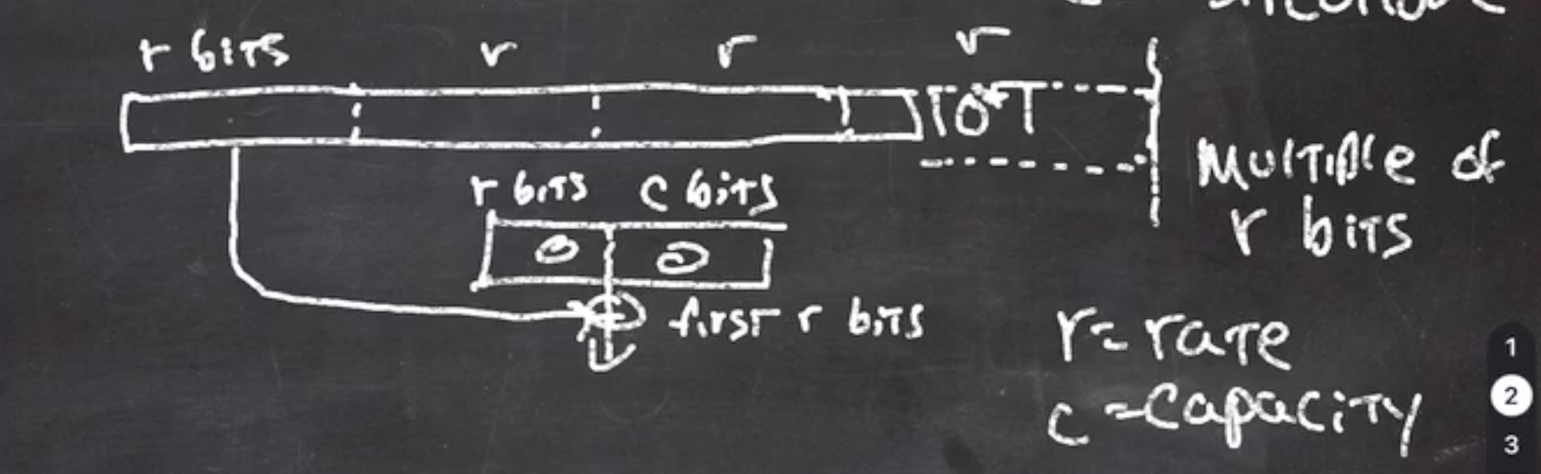This leaves the low \( c \) bits alone.
• the output of this goes through a permutation function \( P \) 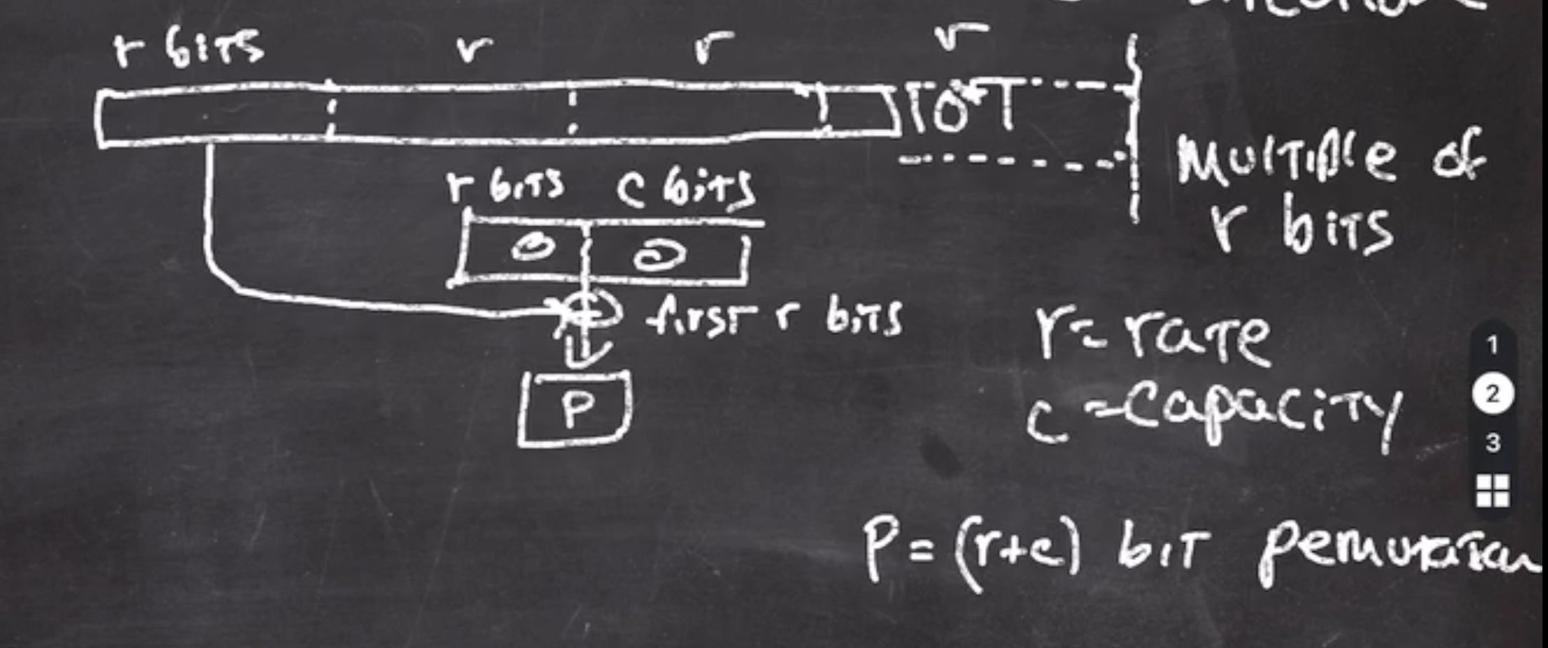\( P \) should be thought of as a public random permutation.
• the output of this is xor’d with the next \( r \) bits of the data, processed through \( P \) , and this continues 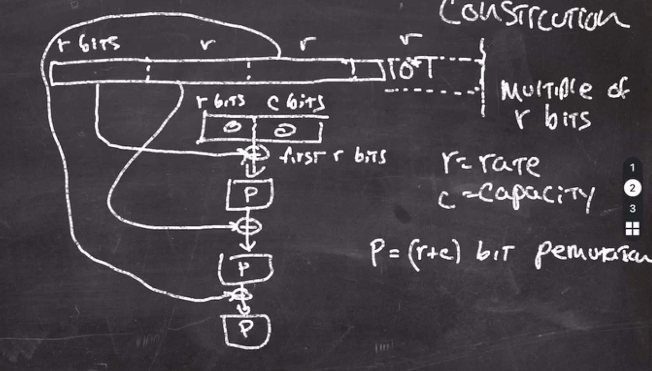This continues until the data is exhausted.
• The output is fed through \( P \) one last time, and the result is the high \( r \) bits of output.

Since the side of \( c \) bits is never touched, nobody has access to manipulating those \( c \) bits. The only way to manipulate the function is to change the bits in \( r \) , which is changing the data.

If our permutation doesn’t output \( r \) bits, it can be called a couple of times until we have \( r \) bits to return.

• The hash function’s speed is effected by how big \( r \) is (which is why we define \( r \) as rate). Each invocation of \( P \) consumes \( r \) bits.
• \( c \) sets the security. An attack will try to cause the \( c \) bits of the block to collide. A secure hash function must have a large enough \( c \) side to make collisions very unlikely. To be secure nowadays, \( c \geq 256 \) .

Consider the last block,

• students often copy the entire data into a buffer that can hold the original data plus the buffered data
  • this is extremely inefficient, imagine a buffer that is 10GB.
• we’ll never have to copy the first multiple of \( r \) bit
  • instead we’ll xor the first \( r \) bits into our chaining value, until we get to the last block
  • for the tail, we’ll use a temporary buffer that is allocated on the stack, and copy the bytes from data then do the 10*1 padding.
  • that way we don’t have to make a copy of the entire data

Later on, when we do a perm384 sponge construction, we will use values of

• \( r = 128 \) bits
• \( c = 256 \) bits

If we want our output to be \( b = 256 \) bits, we will have to call our permutation at the end twice (since our perm384 outputs 16 bytes at a time).

Sponge construction example #

Let \( P : \{0,1\}^6 \to \{0,1\}^6 \) and our permutation function as \( P(x) = \text{ROTL(x,1)} \)

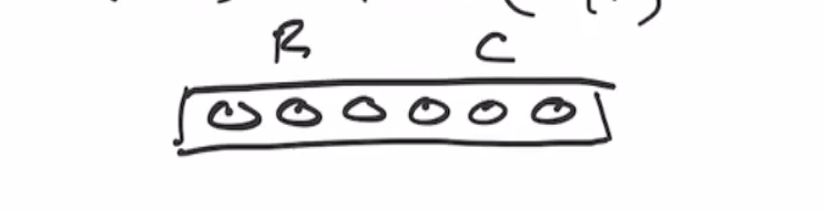
Lets define our rate and capacity as \( r = c = 3 \) .

Recall that the sponge starts as all 0s, split into \( r \) and \( c \) bits:

If we want to hash the value

110011 0101

we’ll need to pad the last block using our 10*1 algorithm,

110011 010111

Note: we always have to add the two 1s when we pad, the 0s are the only thing that is optional.

Next we xor the first 3 bits of our data and xor it with our sponge,

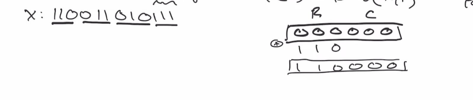
Then we send the sponge through the permutation,

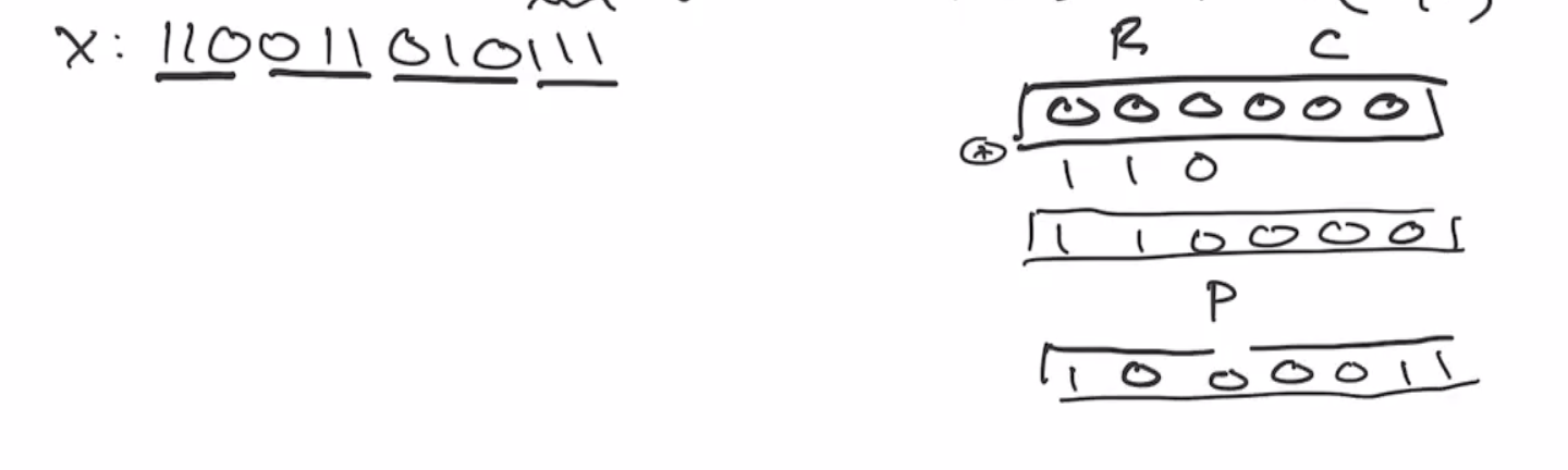
This continues onto the next block of \( r \) bits:

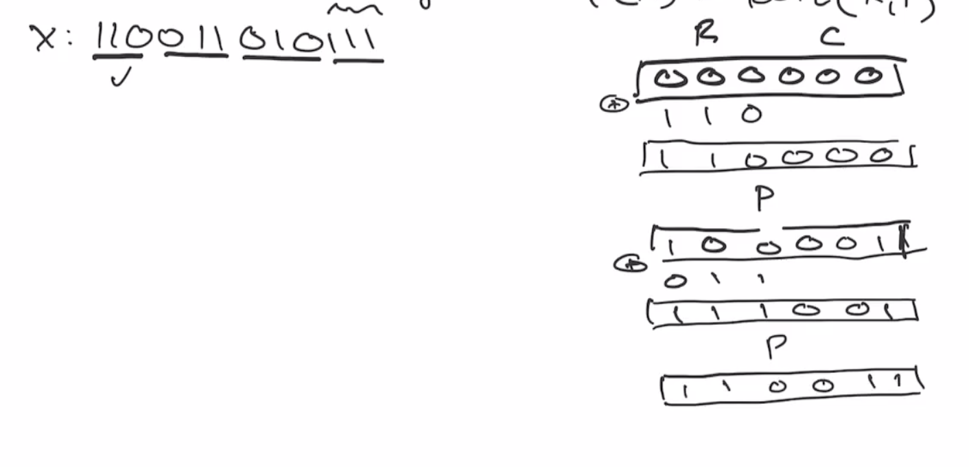
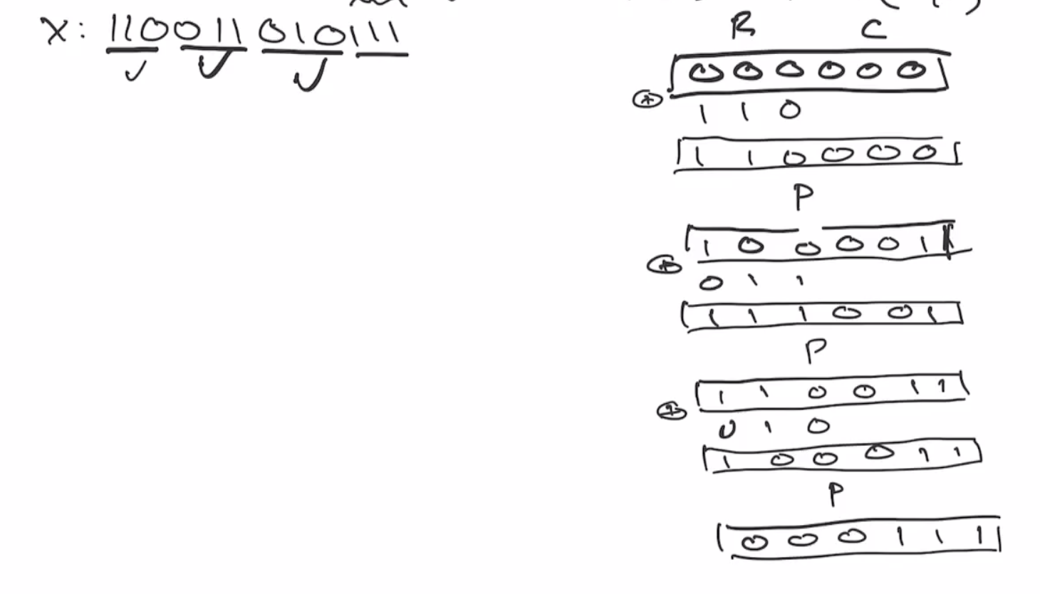
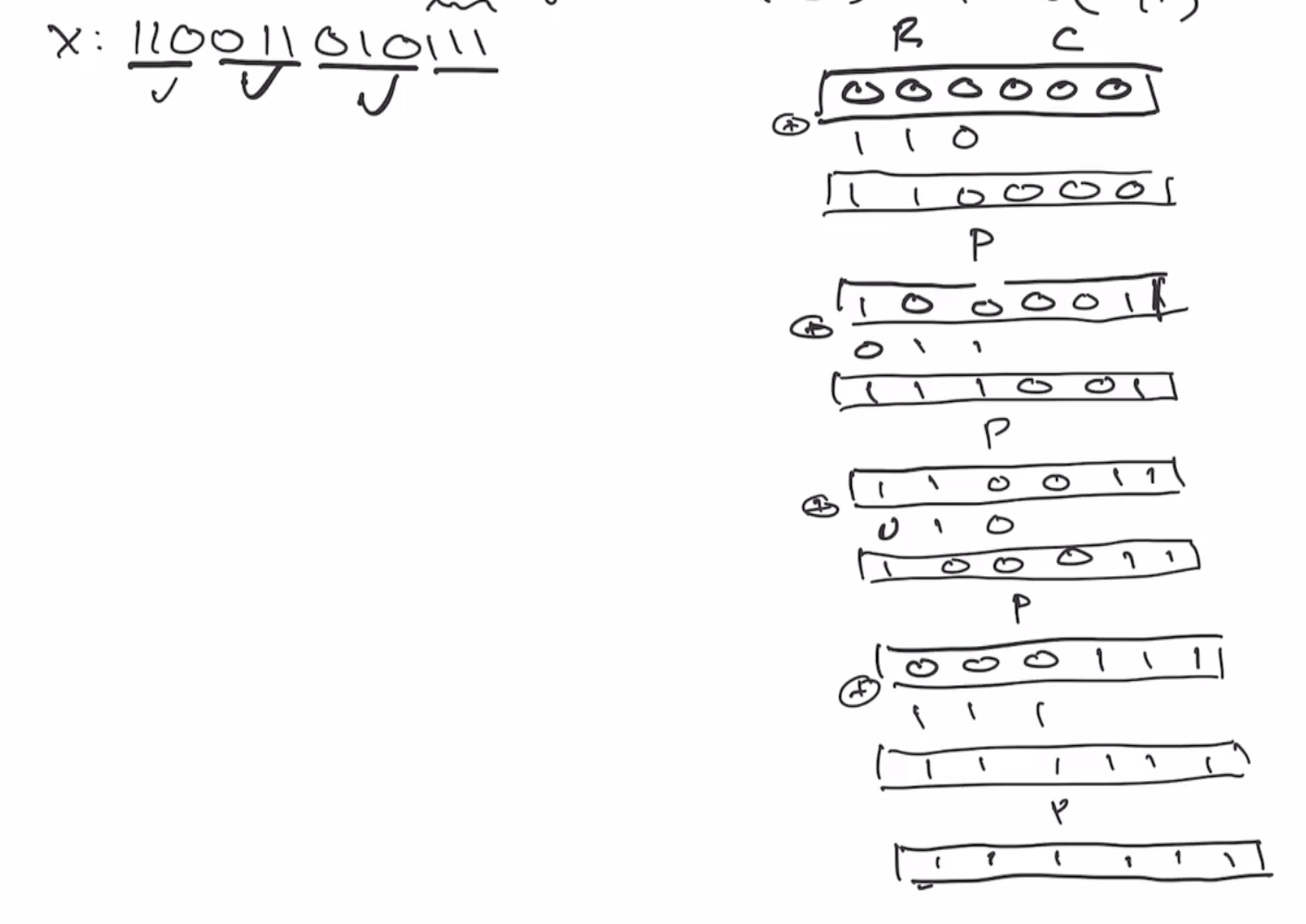
This is the end of the absorbing phase. Next is the squeezing phase, this takes the first \( r \) bits and outputs it as the hash output. So if we want our output to be 6 bits, we’ll outout as many of the \( r \) bits as necessary. So we can output the first \( 3 \) bits, and then send it through the permutation again.

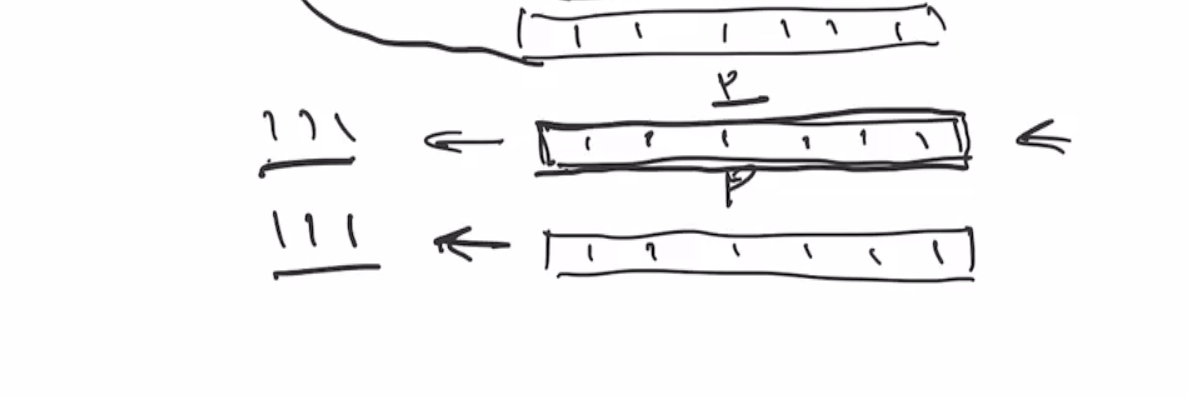
Note: This isn’t the best example because the output of ROTL(111111) is indistinguishable from the input.

Reductions #

If you can write an algorithm that uses a subroutine, like

ASolver(a_inst):
    b_inst = convert_a_to_b(a_inst)
    b_sol = BSolver(b_inst)
    a_sol = convert_b_to_a(b_sol)
    return a_sol

This means that ASolver reduces to BSolver, which means that

“If BSolver exists, then ASolver exists”

These implications do not make any assumptions about the true/false of their existence, it just merely shows an assertion should it exist.

It sometimes happens that we are interested in the constrapositive:

“If ASolver does not exist, then BSolver does not exist”

FindMedian reduction example #

// arr could be in any order
FindMedian(arr):
    arr' = Sort(arr)
    ans = arr'[len(arr') / 2] // assumes odd length arr

This shows that FindMedian reduces to Sort.

Note: If we say FindMedian doesn’t exist, it means that it doesn’t exist for all input.

Reductions in cryptography #

Reductions are important in cryptography because

• one of the ways that cryptographic protocols are proven secure is using these reductions

Since we could use a specific block cipher in an encryption mode, the security of the mode reduces to the security of the block cipher.

CollisionFinder reduction example #

// returns x1 != x2 such that H(x1) = H(x2)
CollisionFinder(H):
    x1 = random string
    x2 = 2ndPreimageFinder(H, x1)
    return (x1, x2)

The contrapositive is a more interesting statement: “Collision resistance implies 2nd preimage resistance.”

There should be an infinite number of \( x_1 \) that map to \( x_2 \) , if the permutation is truly random. But the hash function may not be a perfect permutation, so you could argue to wrap the 2 lines of code in CollisionFinder in a loop. This would change the string and attempt to find new matches.

PreimageFinder example #

CollisionFinder(H):
    do:
        x1 = random string
        y = H(x1)
        x2 = PreimageFinder(H, y) // H(x) = y
    while x2 = NULL or x1 = x2
    return (x1, x2)

“Collision resistance implies preimage resistance.”

So this displays that the ultimate goal should be collision resistance, because it will also cover preimage/2nd preimage resistance.

Universal hashing #

Compared to cryptographic hashes, which are over engineered for security, universal hashes are a lot more efficient. We don’t always need collision resistance and random looking output. What we sometimes need is a bound on the probability that the adversary could find a pair of inputs that produce the same output.

We can optimize universal hash functions to meet the goals needed.

Its good to note that universal hashes are

• fast, and
• provable to have a small probability to find collisions

This last point when compared to cryptographic hash functions: cryptographic hash functions are overengineered and have so many heuristics that its harder to prove the probability of collisions.

Universal hash functions do not have as much guarantee of the crypgoraphic hash functions, but if all we need is the probabilistic property, then they are the way to go.

Abstract epsilon universal hash example #

Let \( H \) be a collection of hash functions \( A \to B \) , (from some domain \( A \) to a codomain \( B \) ). \( H \) is \( \epsilon \) -almost-universal if the probability of winning the following game is \( \leq \epsilon \) .

The game is described as

1. Adversary chooses \( a \) and \( b \) , where \( a \neq b \in A\) .
2. \( h \in H \) is chosen randomly. (Note, the adversary knows the functions in \( H \) but doesn’t know which one has been picked.)

• Adversary wins if
  • \( h(a) = h(b) \)

Concrete universal hash example #

Consider this mapping \( Z_6 \to Z_4 \) :

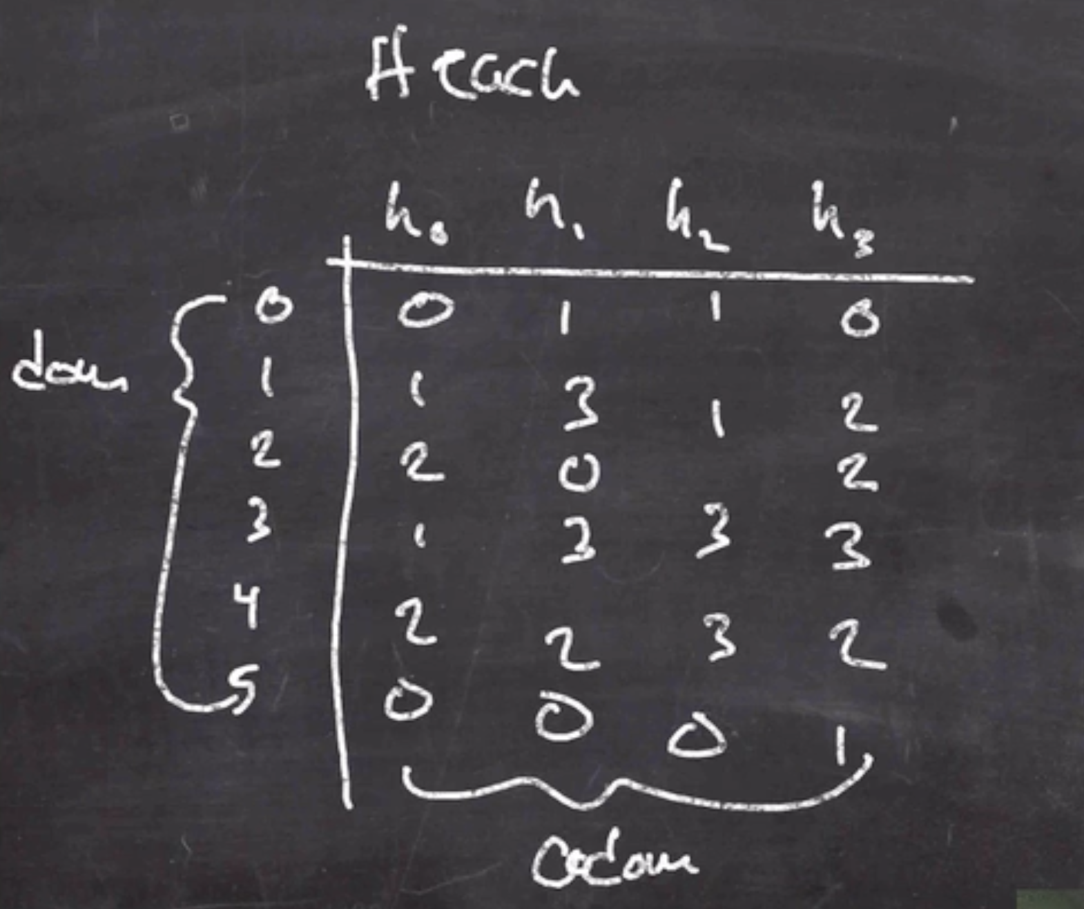
This is a small enough sample of objects that we can calculate the probability of winning the game:

• \( (0,1) = \frac{1}{4} \)
• \( (0,2) = 0 \)
• \( (0,3) = 0 \)
• \( (0,4) = 0 \)
• \( (0,5) = \frac{1}{4} \)

We can continue to go through these pairs until we find a probability that is better than \( \frac{1}{4} \) , for example

• \( (1,3) = \frac{1}{2} \)
• \( (2,4) = \frac{1}{2} \)

Since we can win this game, no more than \( \frac{1}{2} \) the time, we consider it to be \( \epsilon \) -almost-universal for \( \epsilon = \frac{1}{2} \) .

So the smaller the epsilon \( \epsilon \) , the less probability of a collision.