Sensitivity analysis cont. #

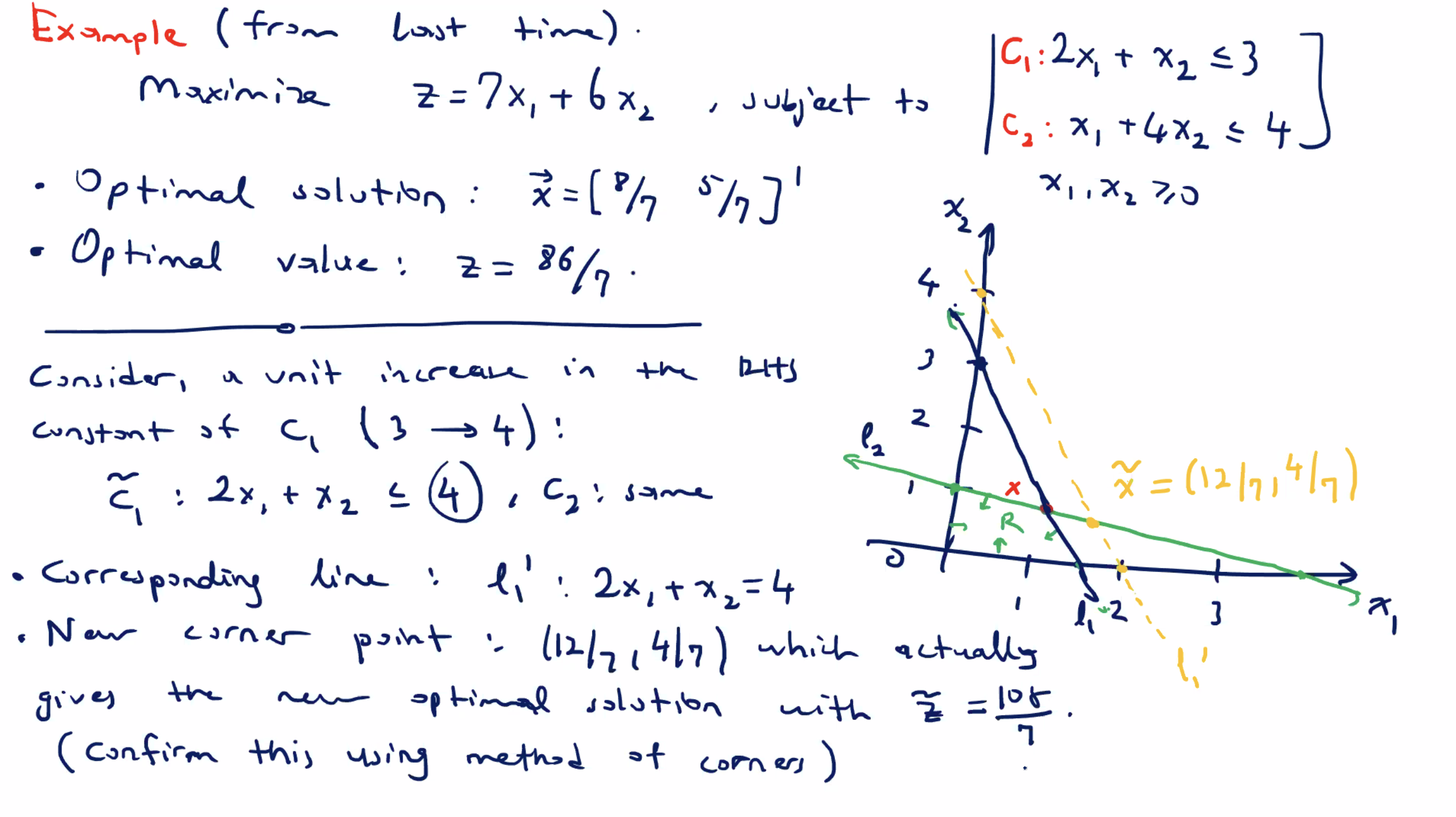
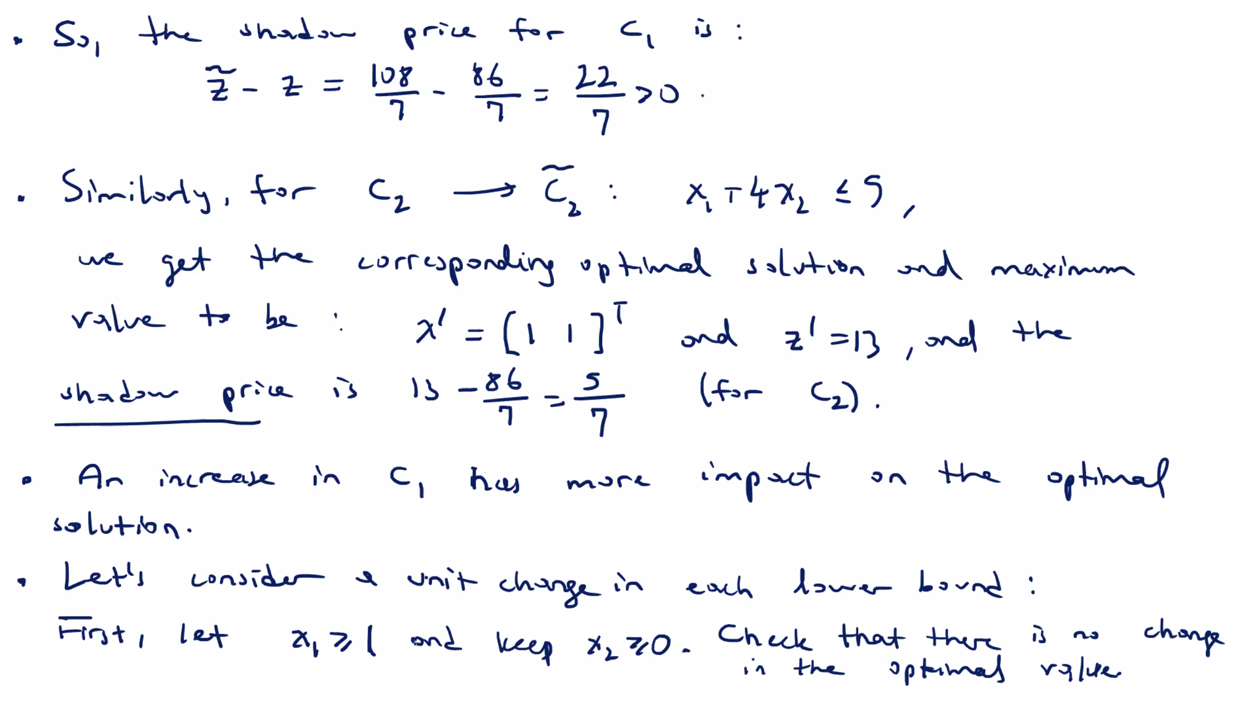
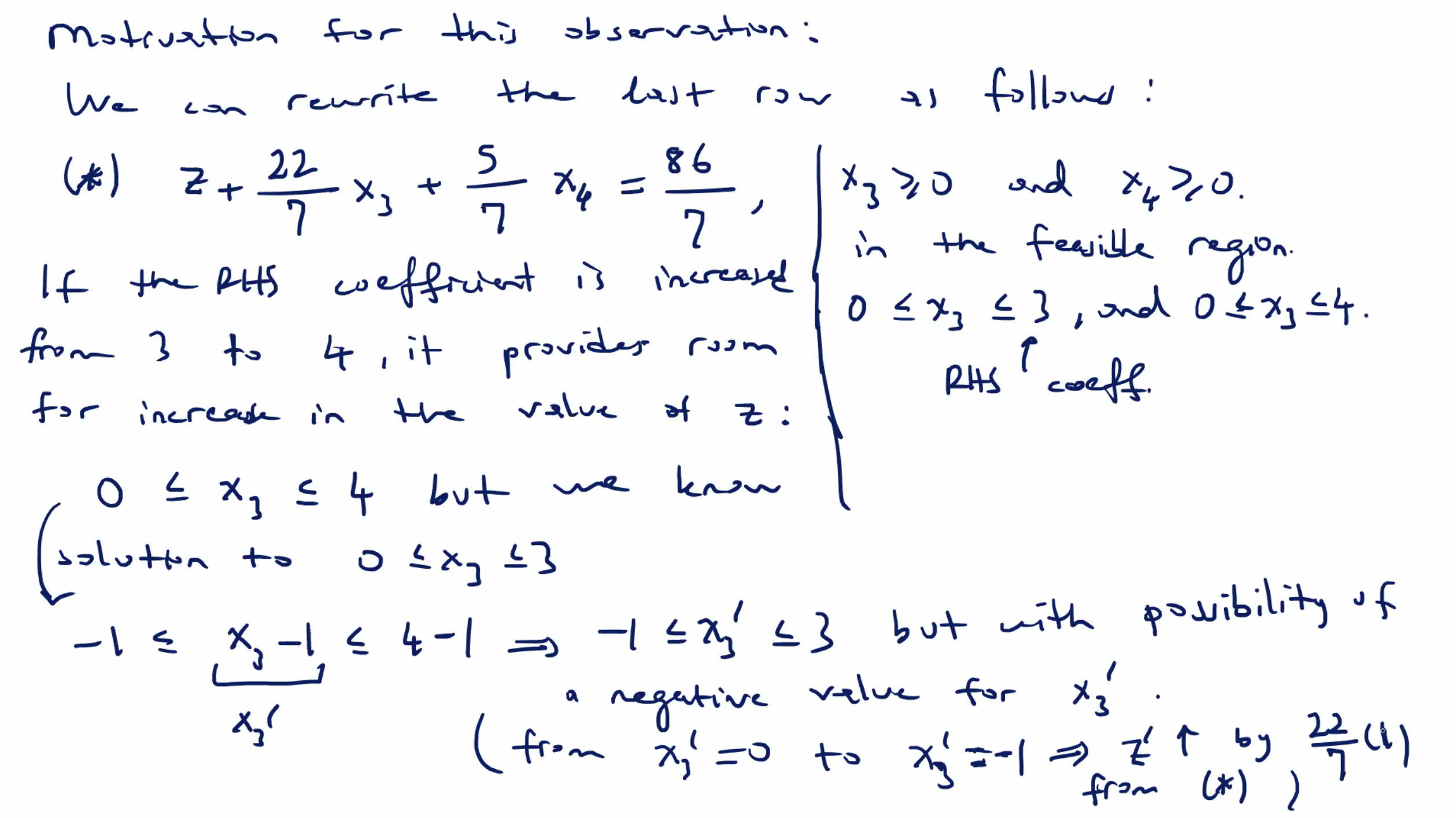
By increasing the right hand side of the \( c_1 \) constraint by 1 unit, we obtain a new \( \tilde{z} \) value of \( \frac{108}{7} \) .

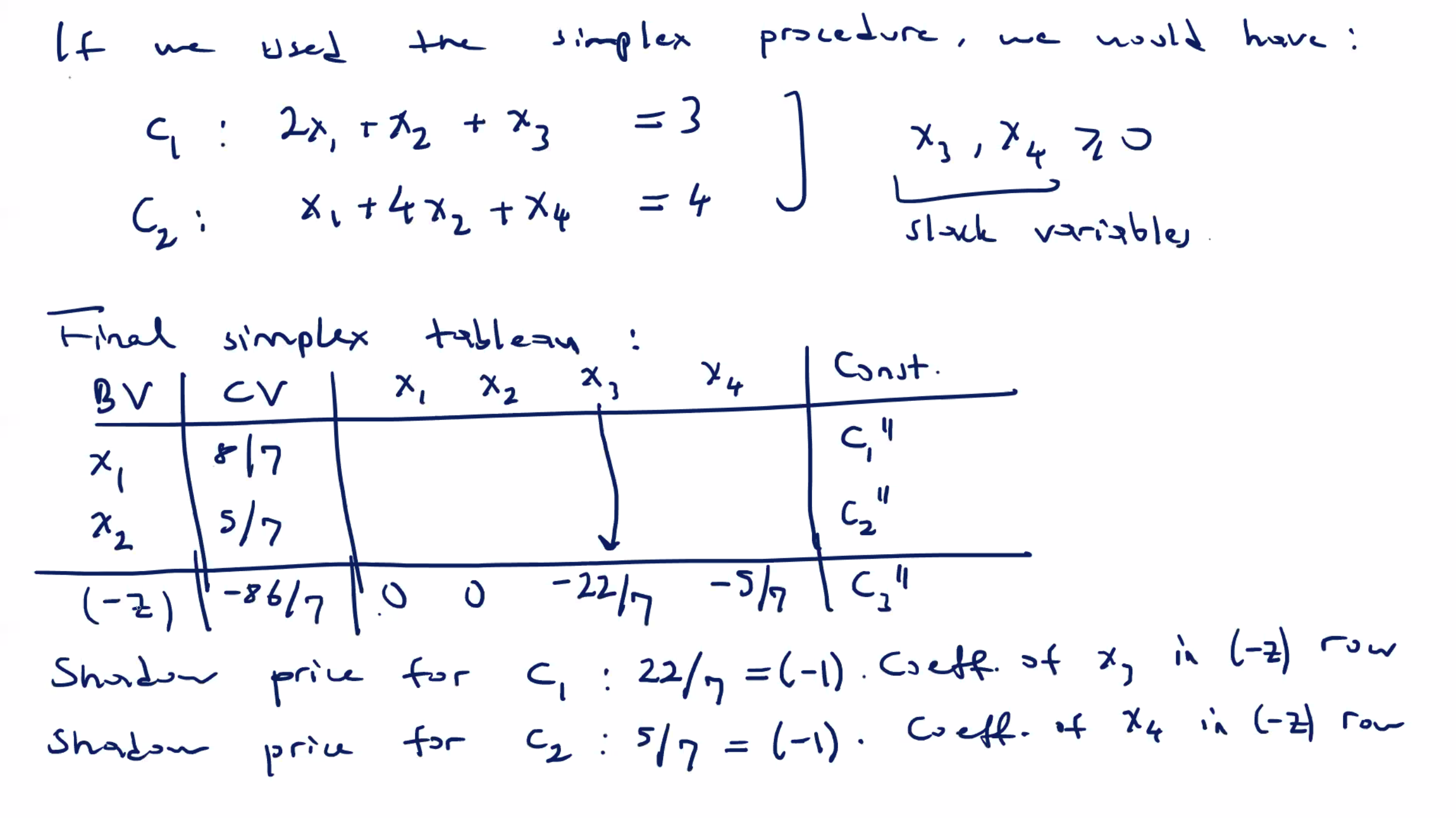
So the shadow price is \( z - \tilde{z} = \frac{22}{7} \) .

Next, identify shadow prices from a completed simplex tableau:

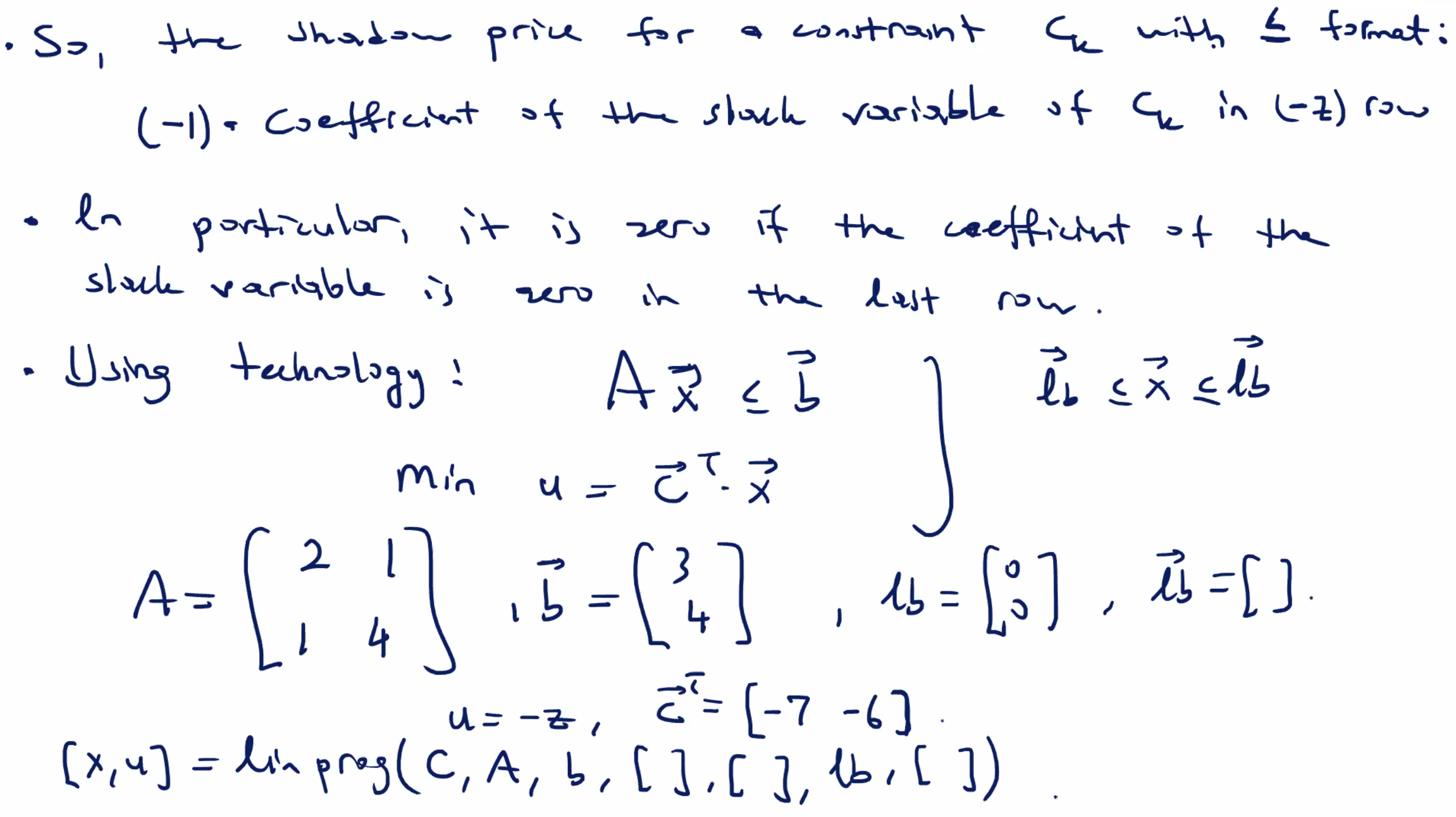
Shadow prices using MATLAB #

A=[2 1; 1 4]
b=[3 4]'
C=[-7 -6]'
lb=[0 0]'

[x, u]=linprog(C,A,b,[],[],lb,[])

Optimal solution found.

x =
    8/7
    5/7

u = 
    86/7

Then we can start playing with the constraints to see shadow prices.

b1=b
b1(1)=4
[x, u1]=linprog(C,A,b1,[],[],lb,[])

Optimal solution found.

x =
    12/7
    4/7

u =
    -108/7

b2=b
b2(2)=5
[x, u2]=linprog(C,A,b2,[],[],lb,[])

Optimal solution found.

x =
    1
    1

u2 =
    -13

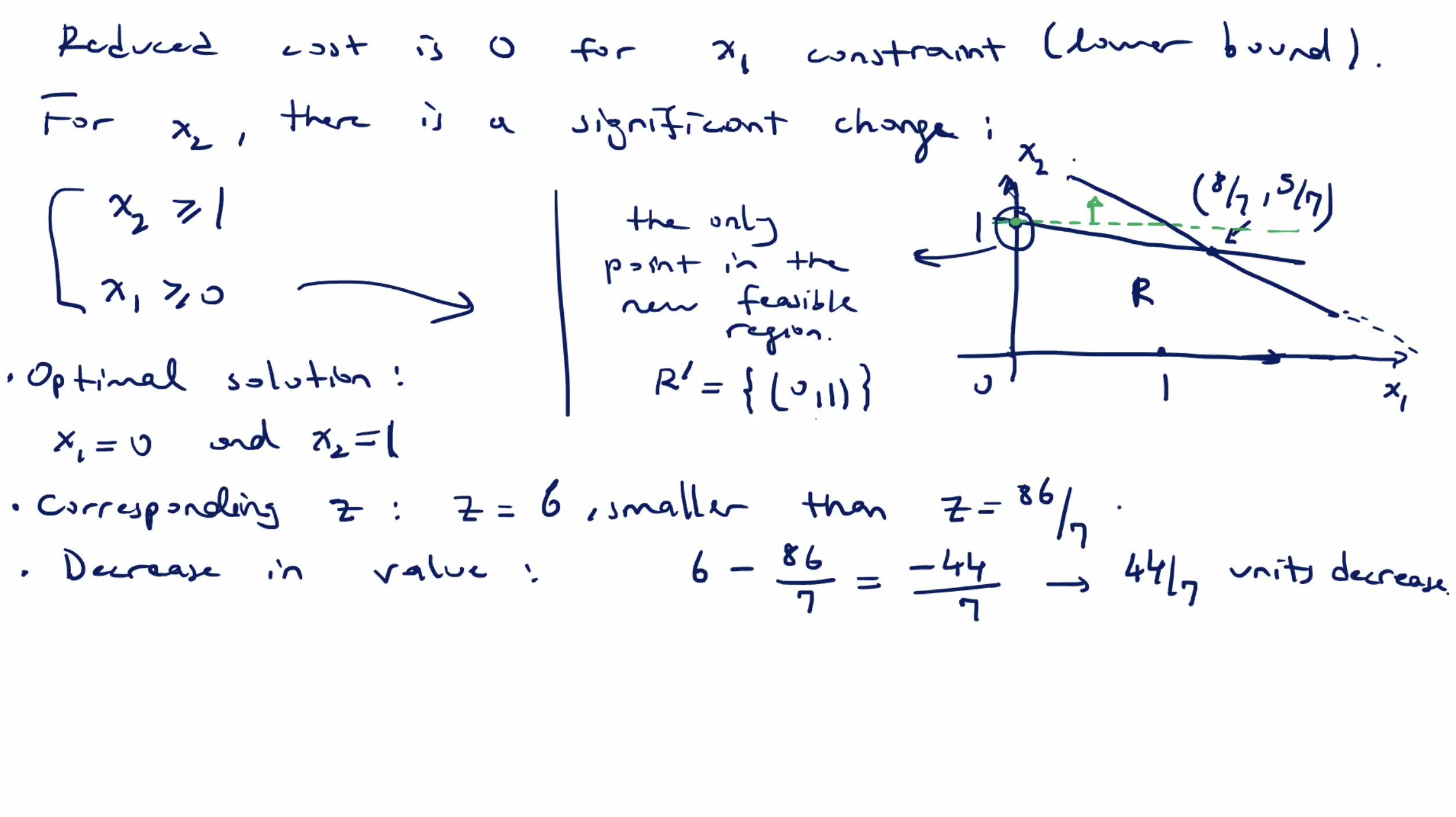
lb1=[1 0]
[x, u3]=linprog(C,A,b,[],[],lb1,[])

Optimal solution found.

x =
    8/7
    5/7

u3 =
    -86/7

Exercise #