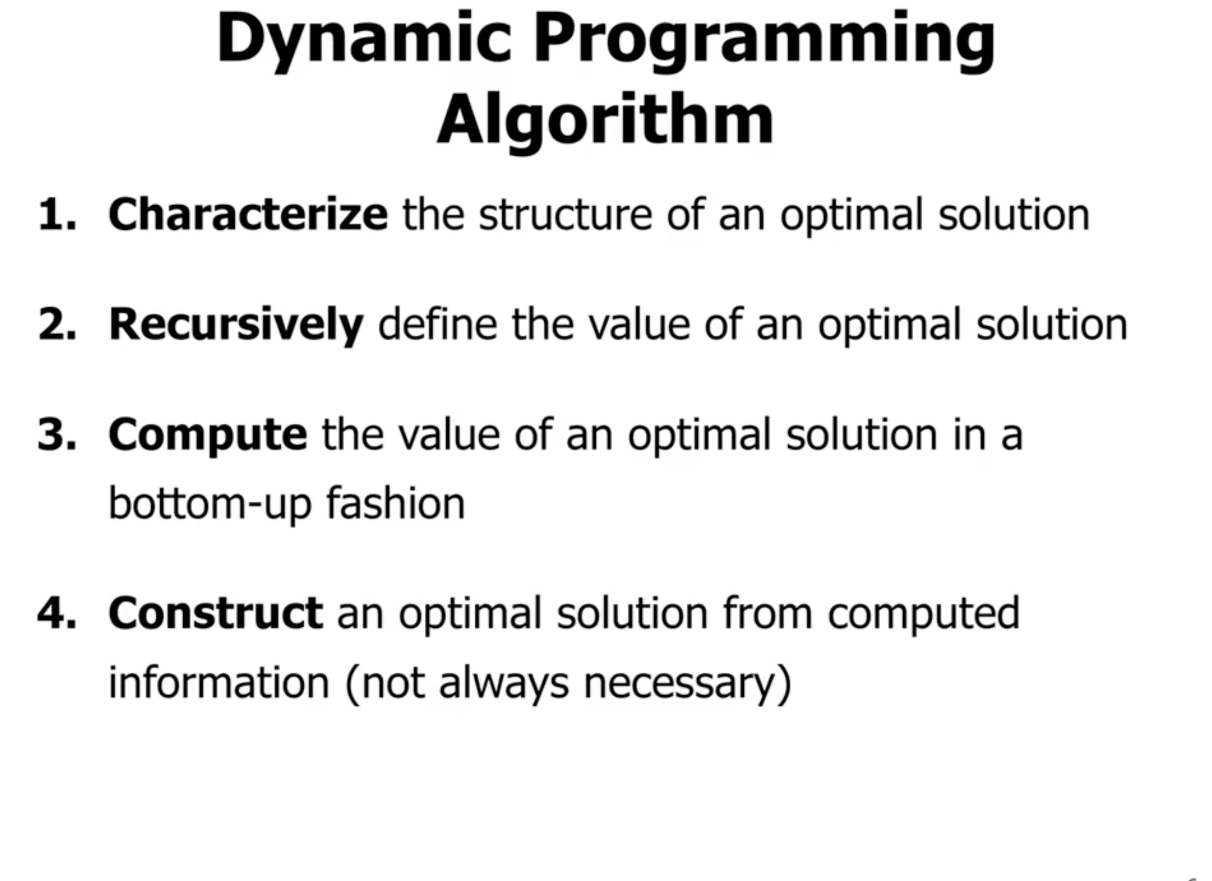
Dynamic programming #
Dynamic programming is an algorithm design technique. In dynamic programming, you solve the problem bottom-up (as opposed to top-down in divide and conquer).
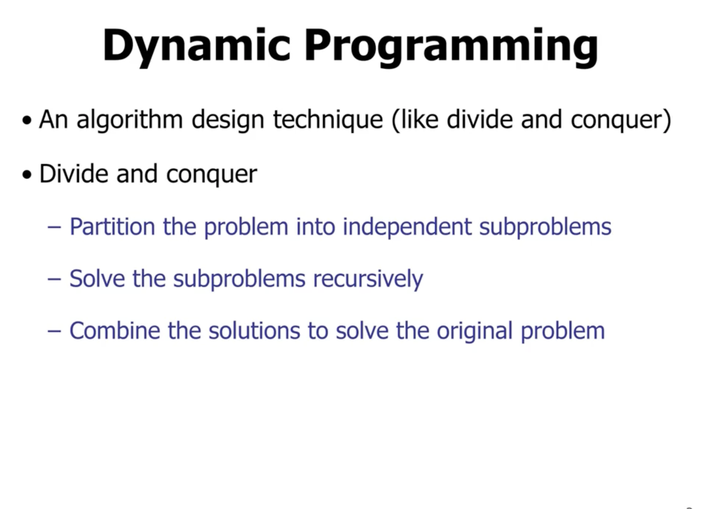
Another trait of dynamic programming is that when a sub problem is solved, it is only solved once (which may not be the case in divide and conquer).
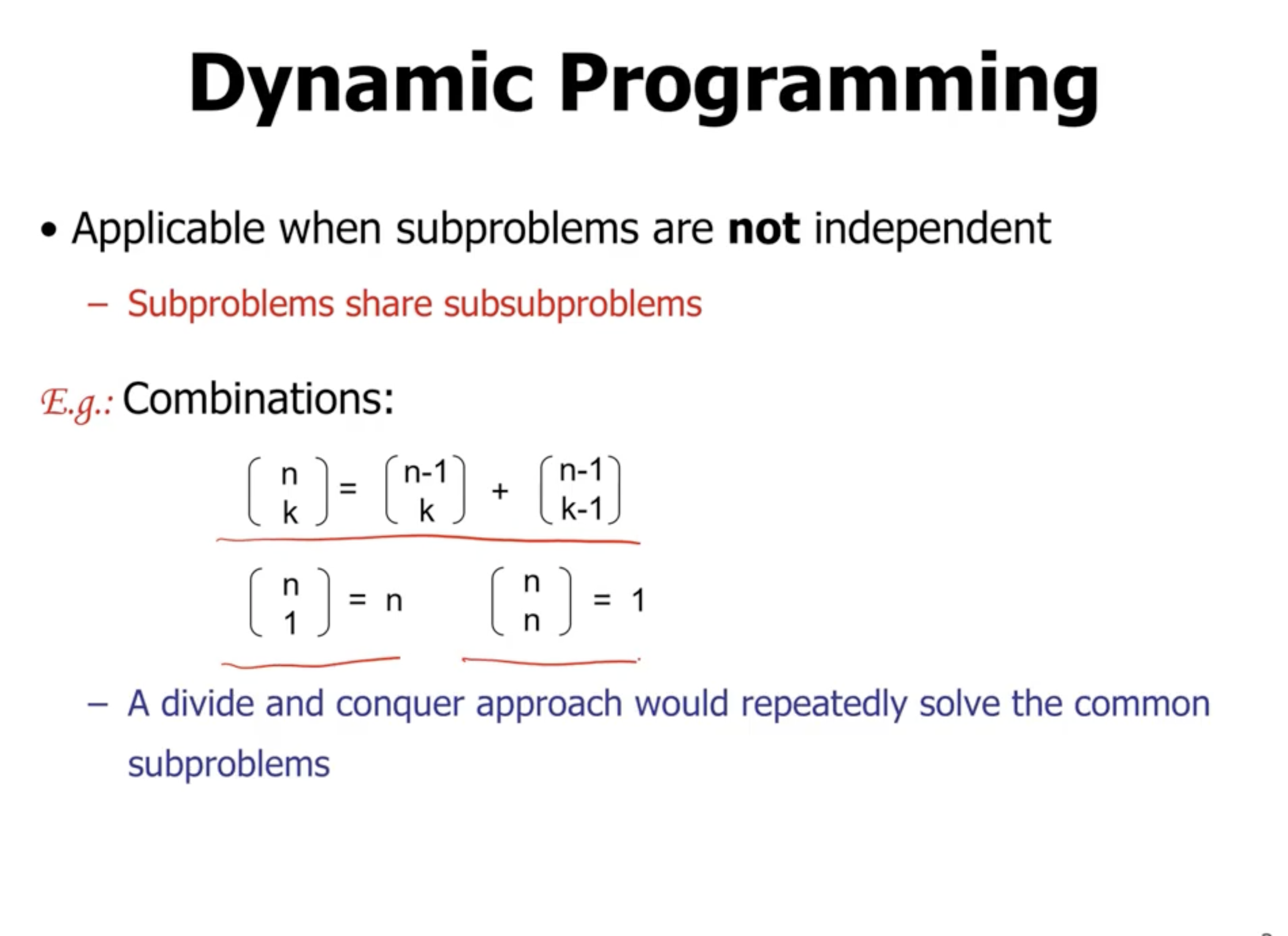
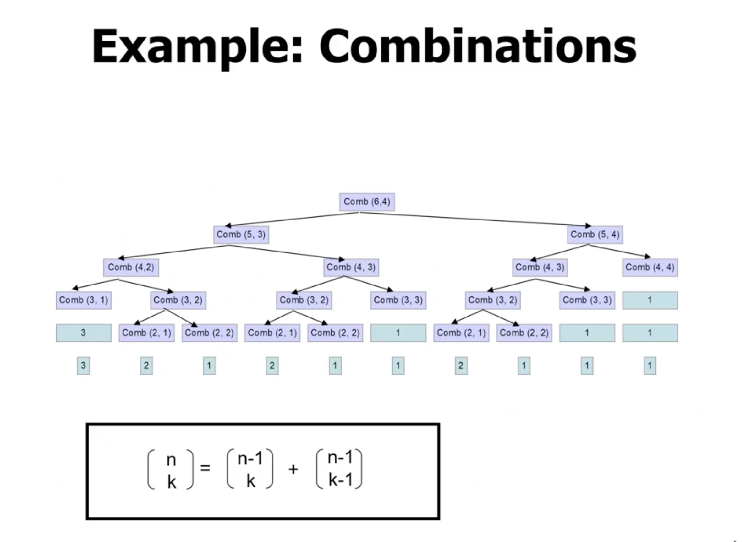
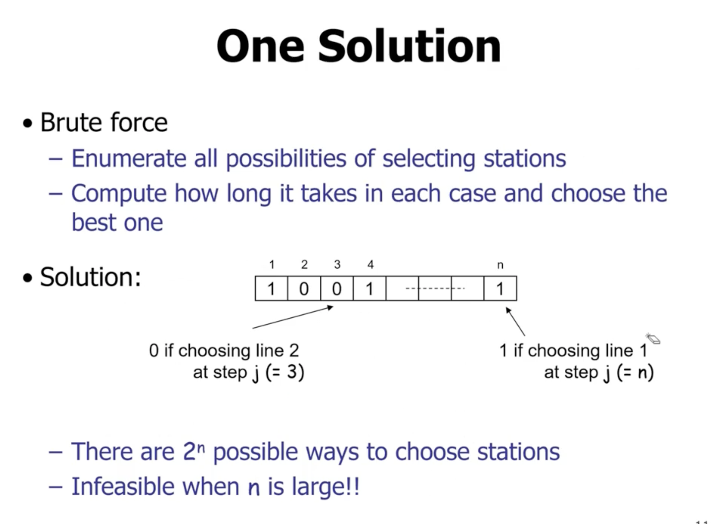
- Notice that multiple sub problems are solved multipled times
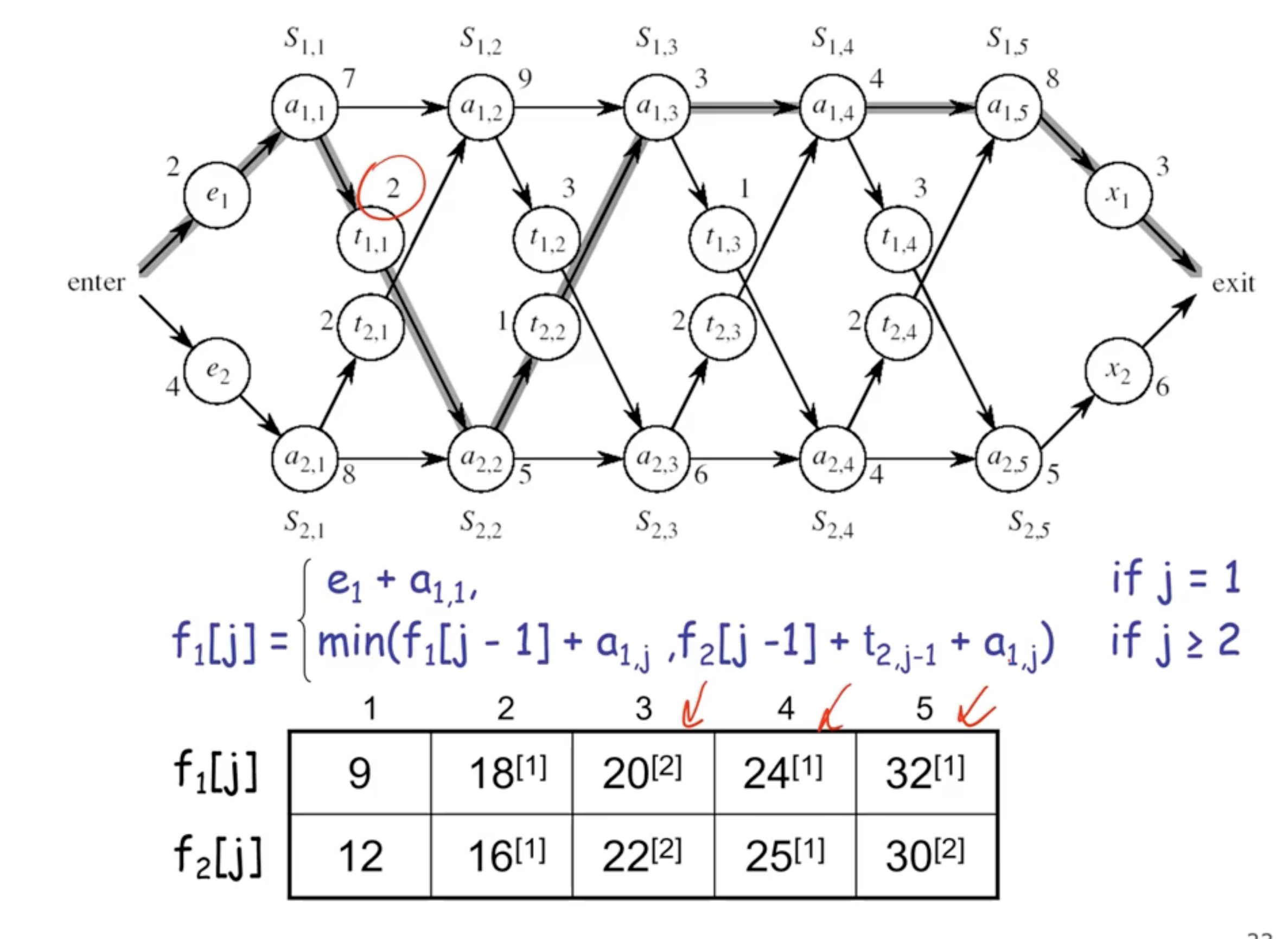
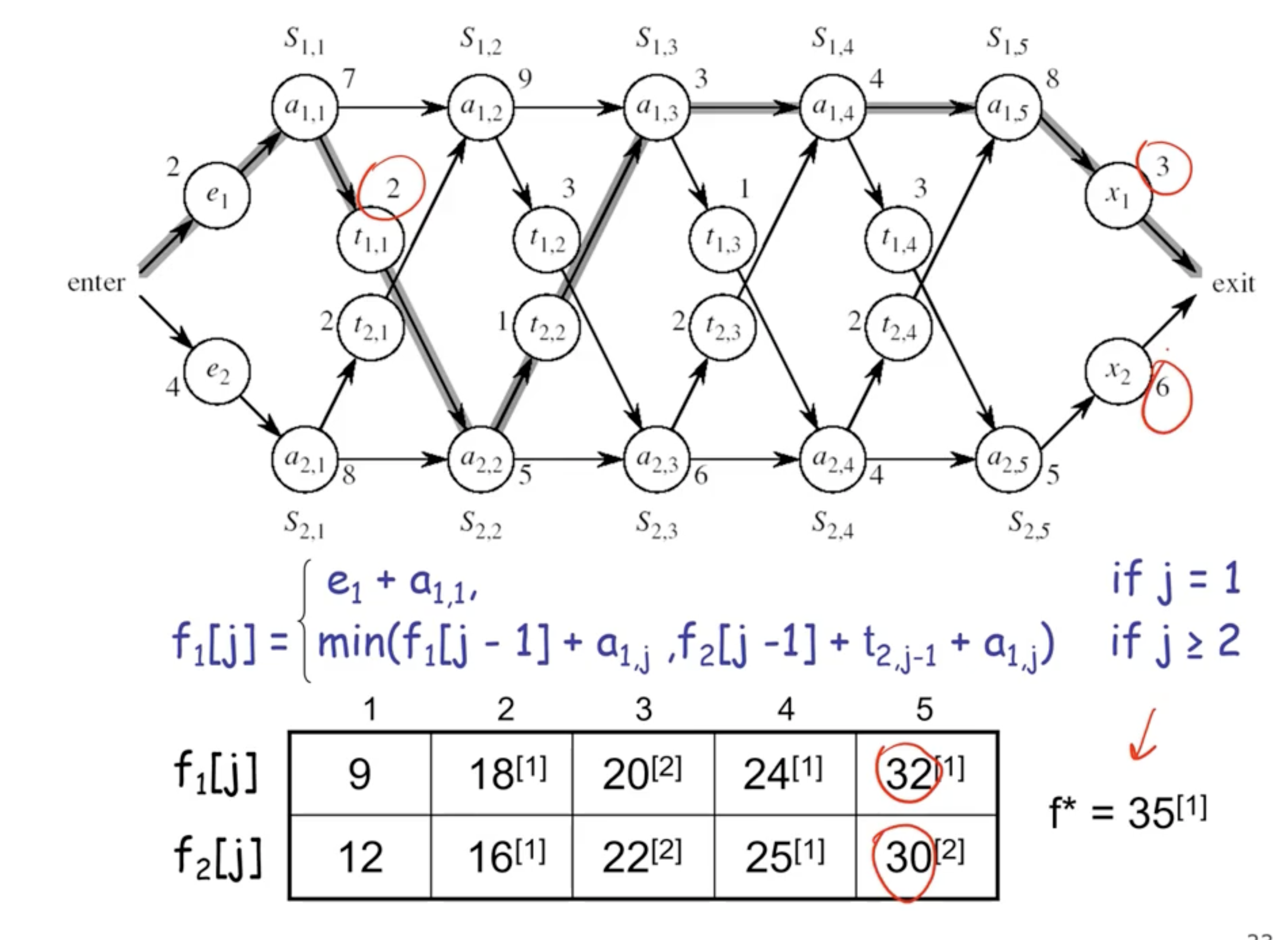
Assembly line scheduling problem #
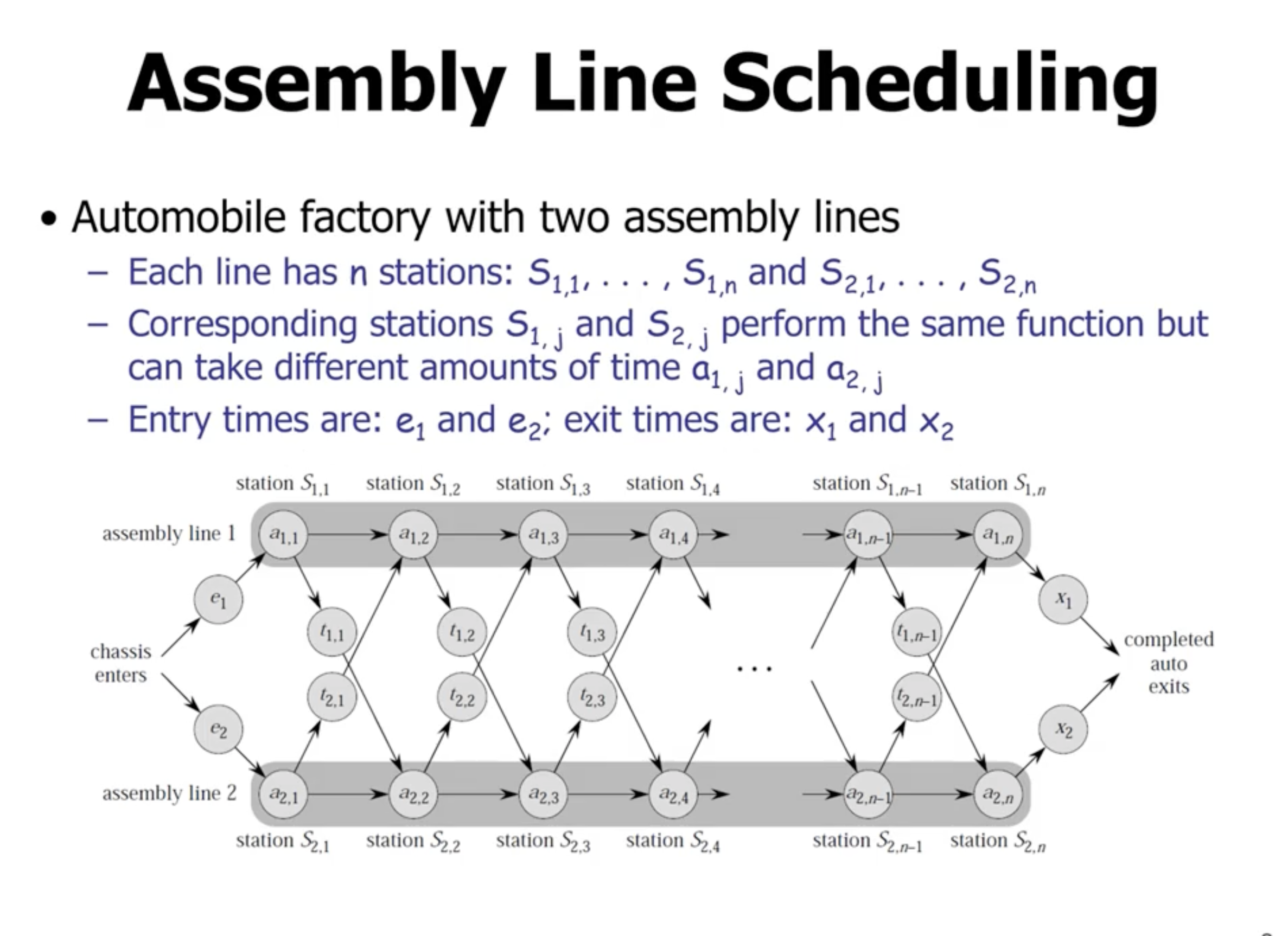
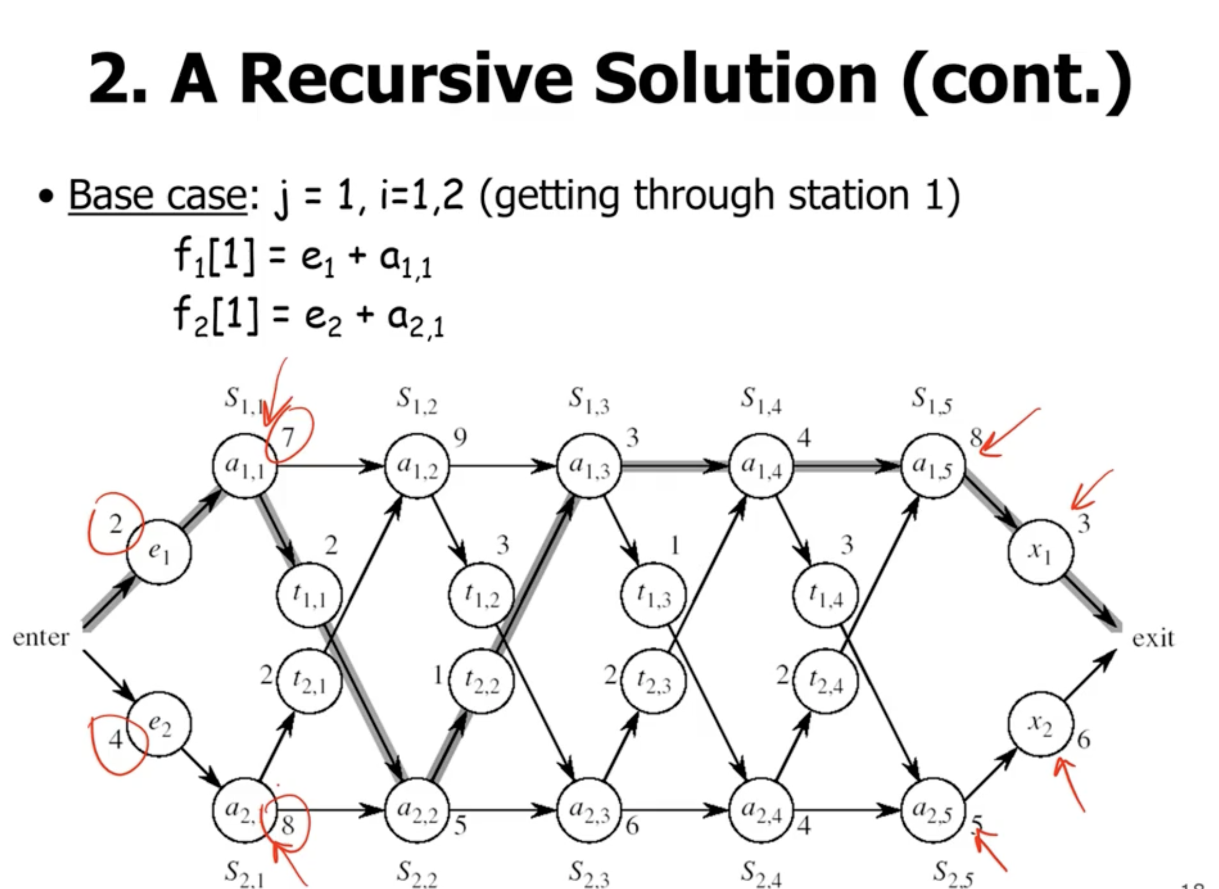
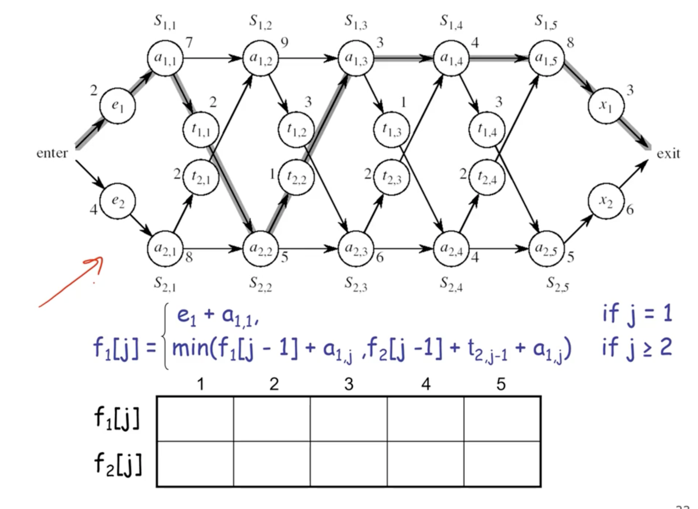
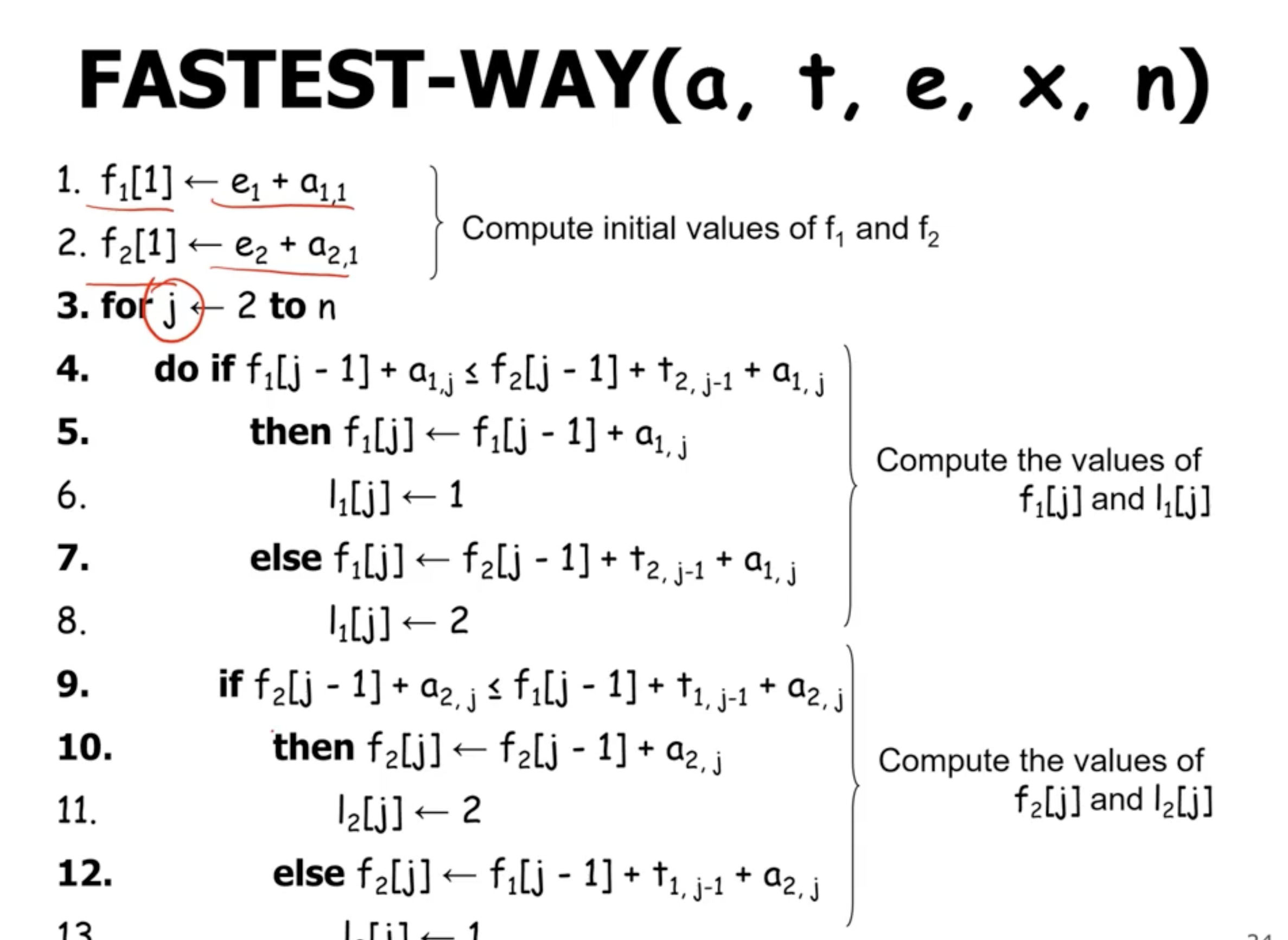
- \( e_n \) is the arrival time in assembly line \( n \)
- \( a_{i,j} \) is the time it takes at station \( j \) in assembly line \( i \)
- \( t_{i,j} \) is the transfer time
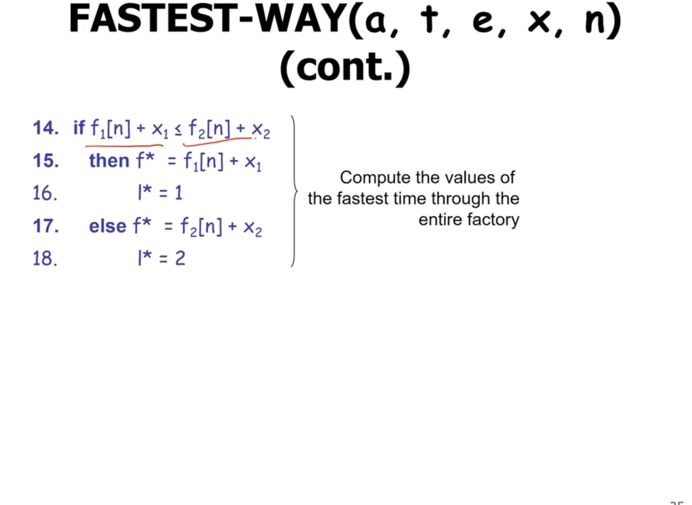
- \( x_n \) is the exit times for assembly line \( n \)
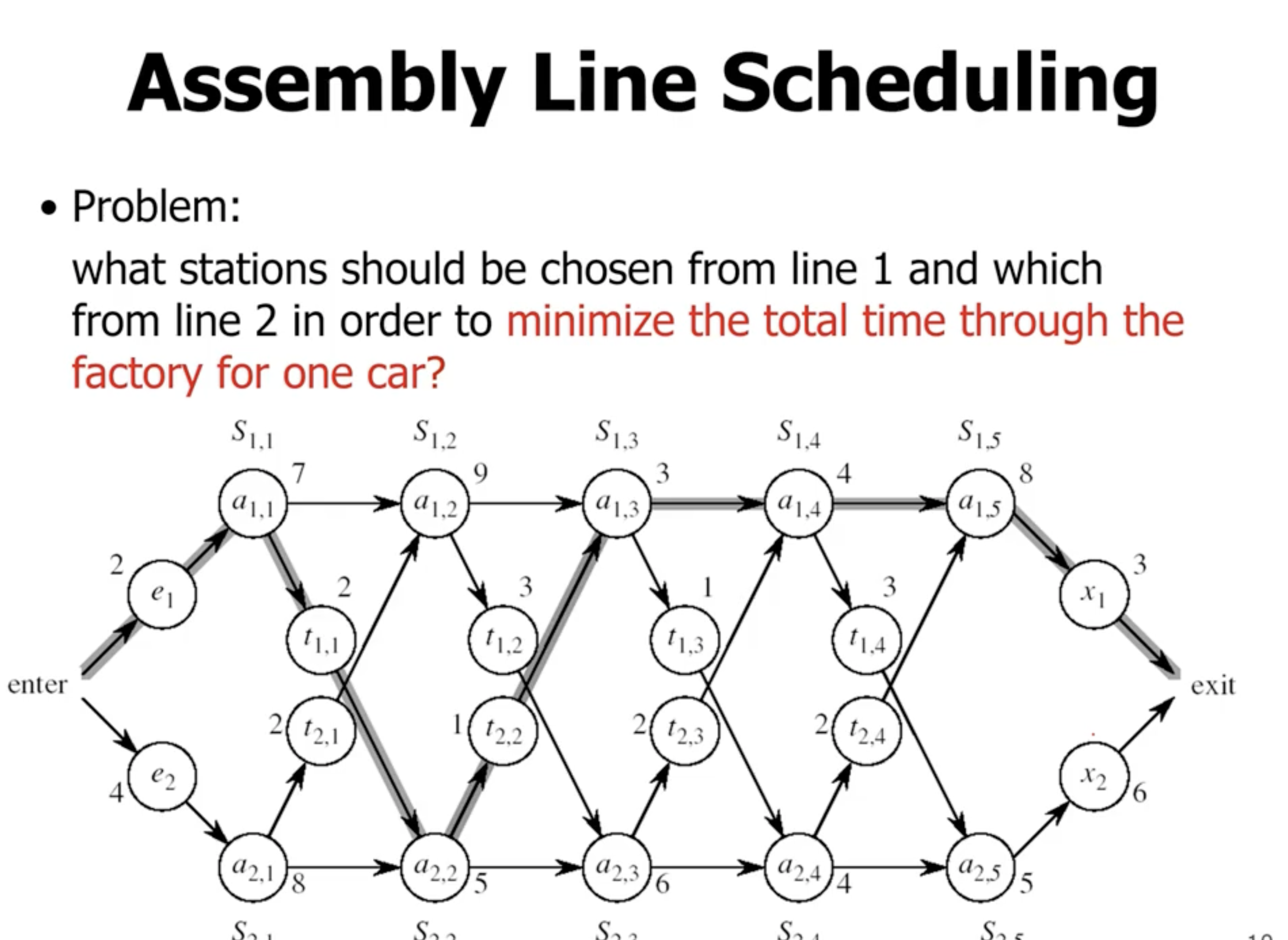
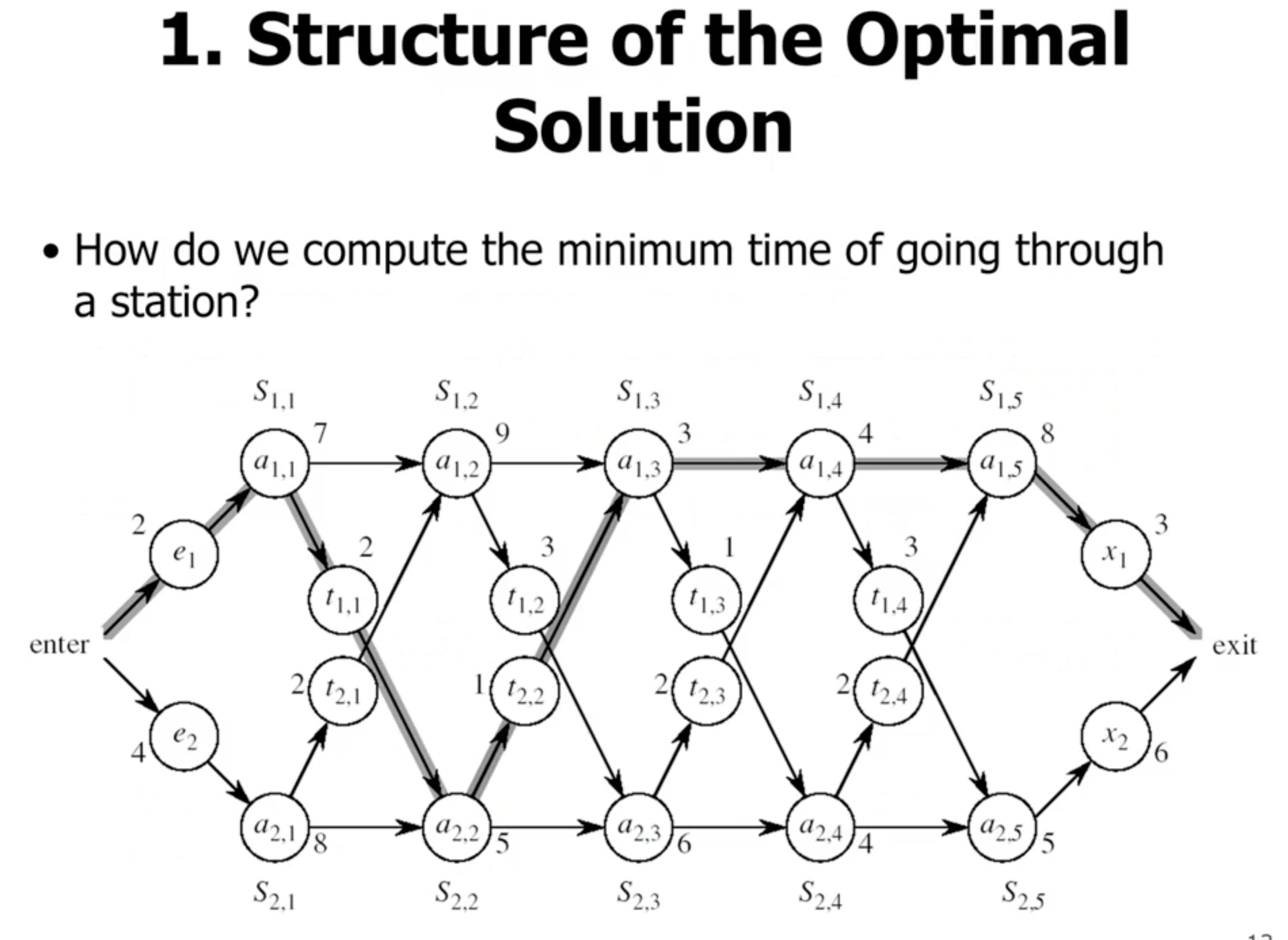
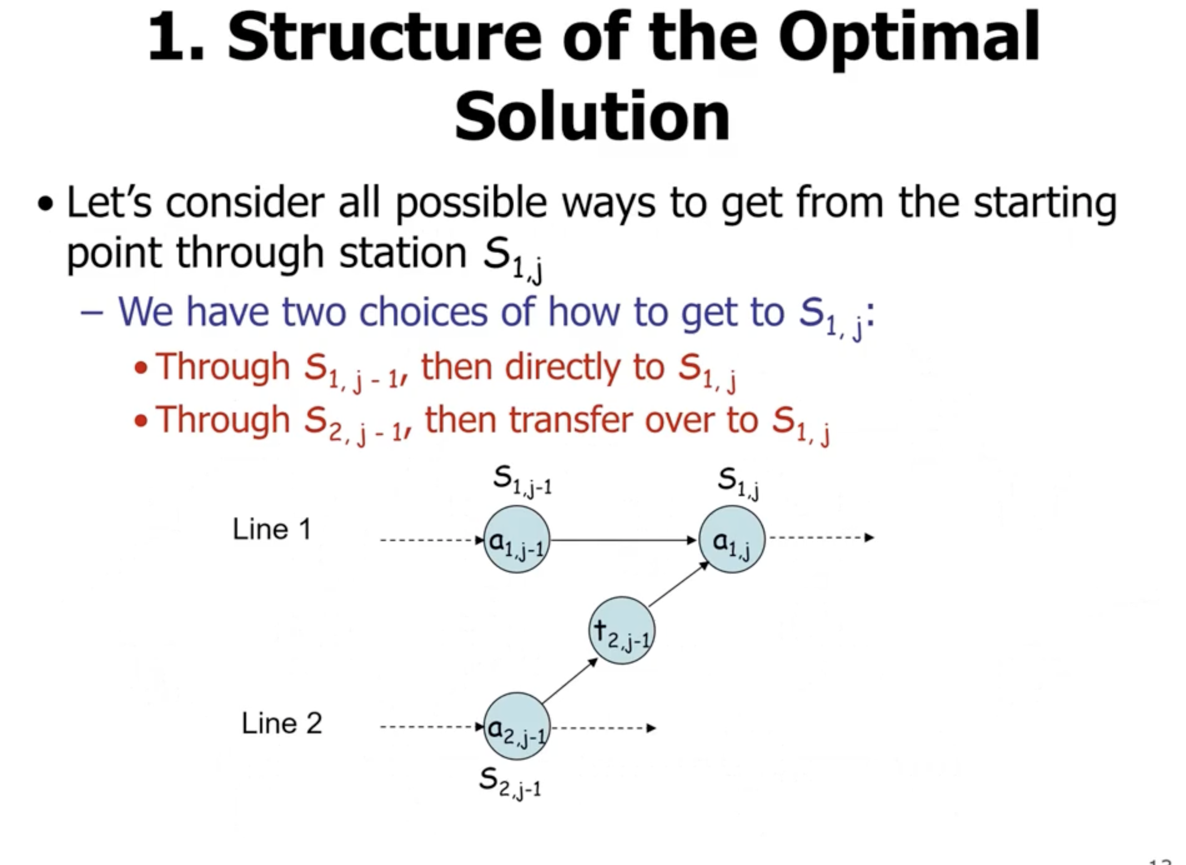
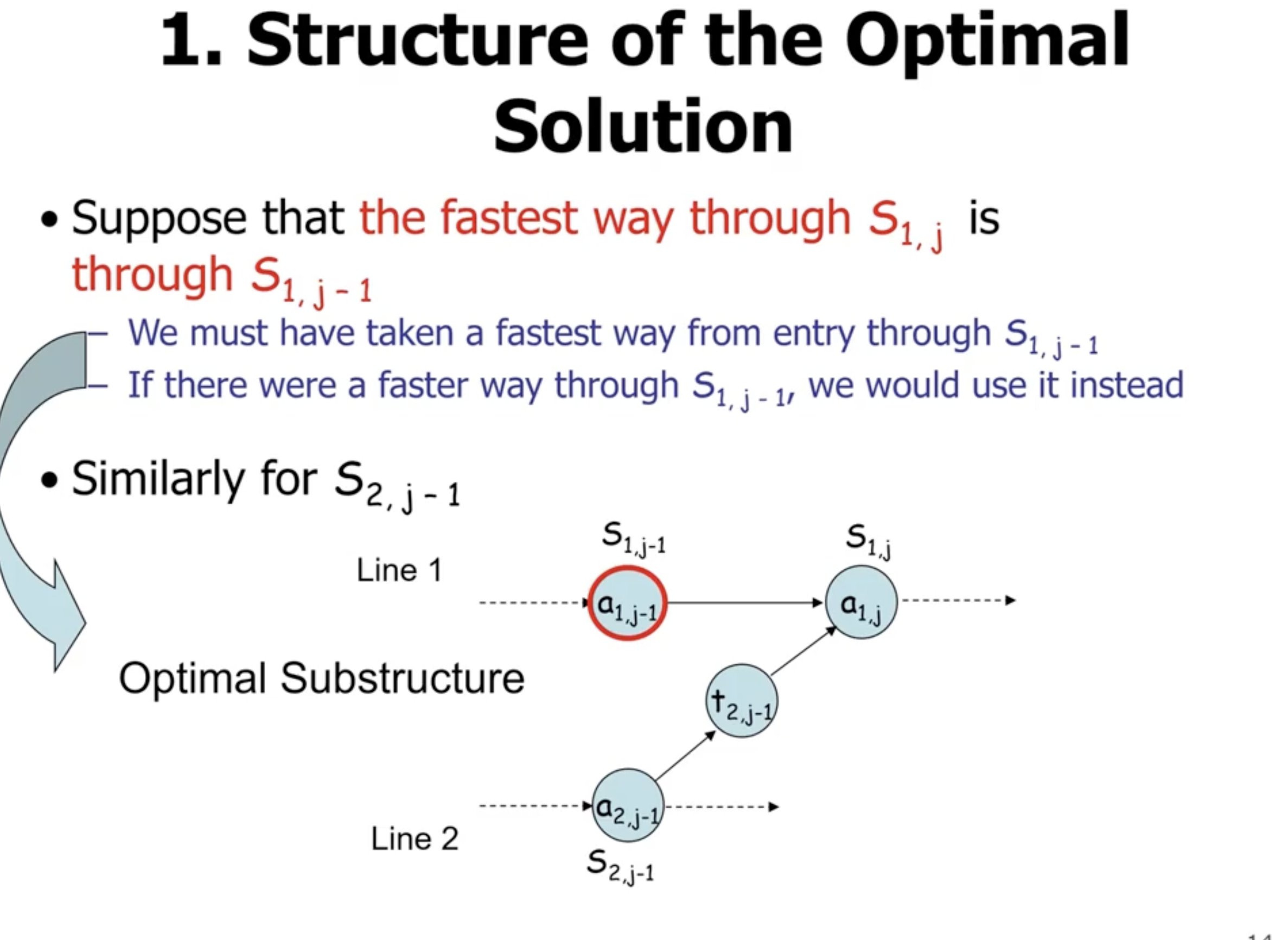
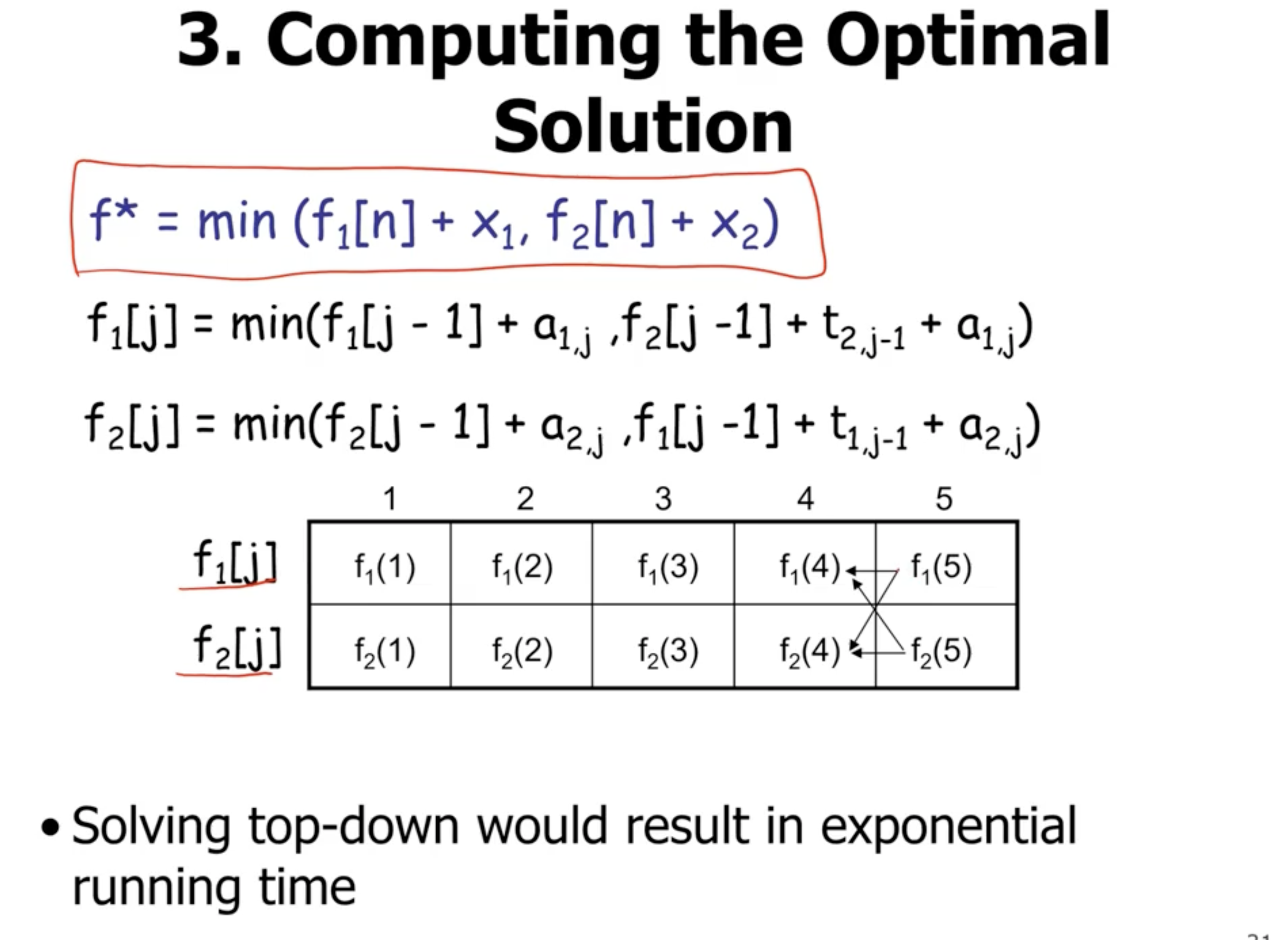
- the idea is that \( a_{1,j} \) has the optimal subproblem solution to \( a_{1,j-1} \) and the optimal subproblem solution to \( a_{2,j-1} \) in it
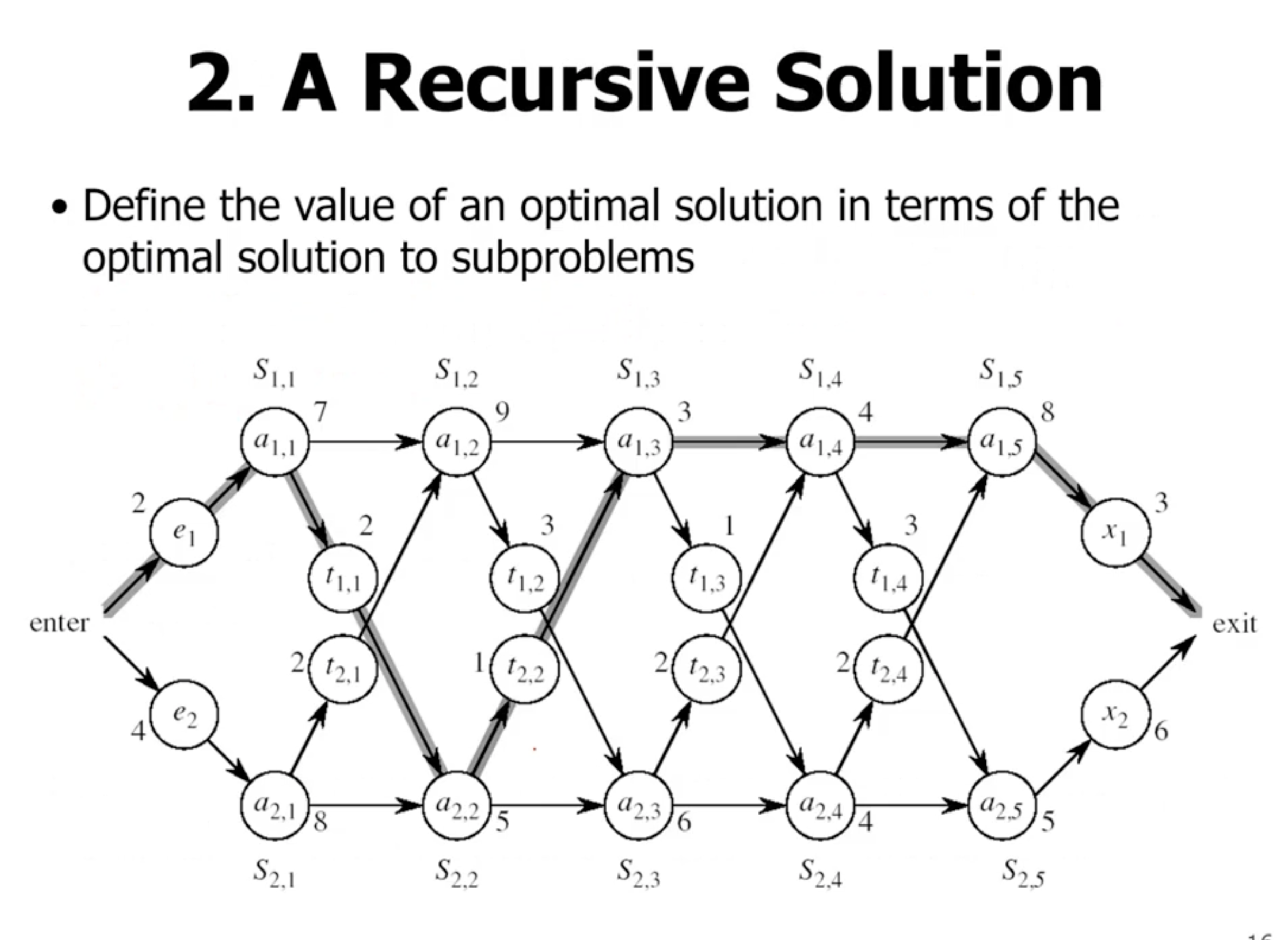
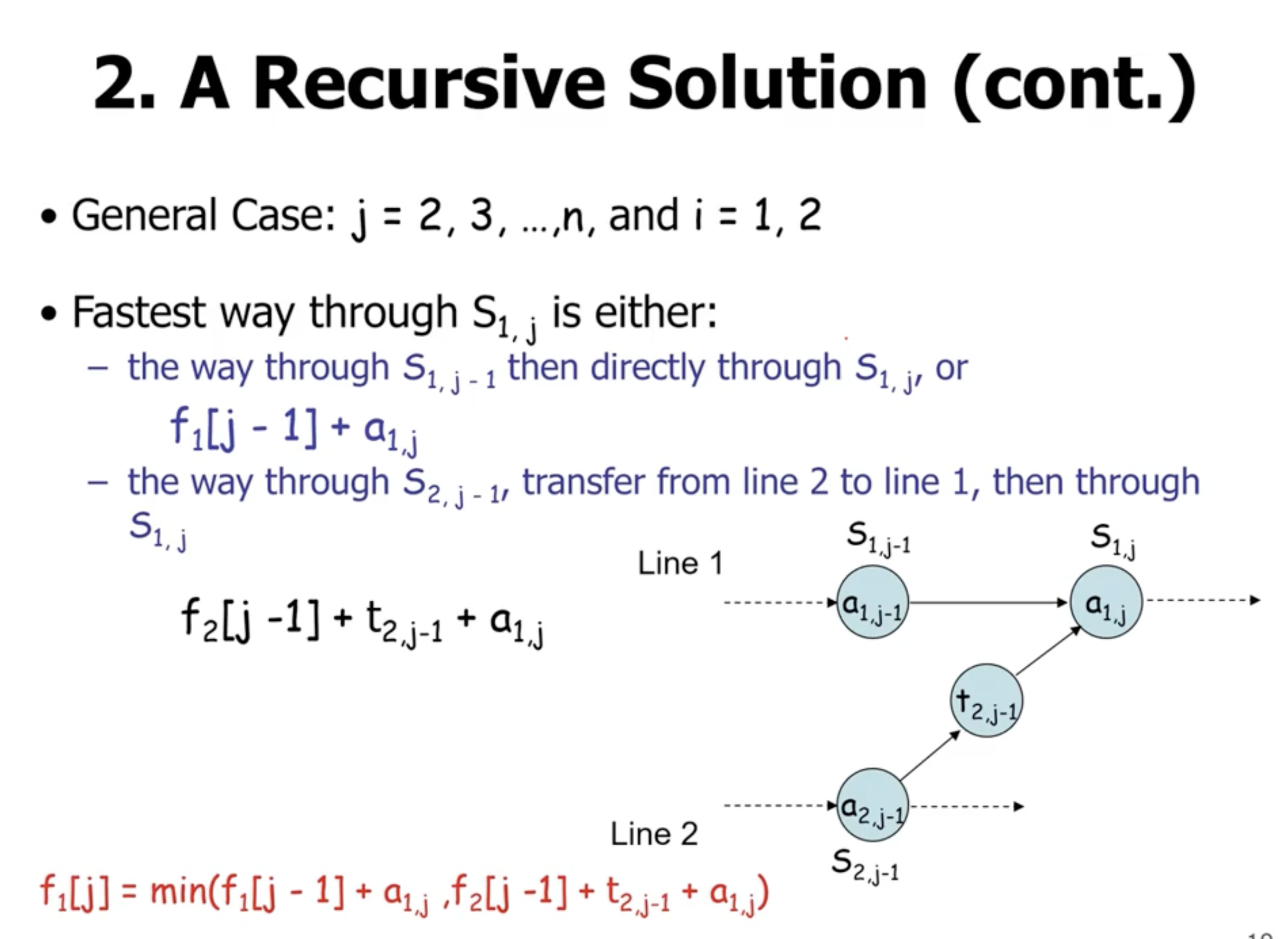
So in general
\[\begin{aligned} f_1[j] &= \text{min}(f_1[j-1] + a_{1,j}, f_2[j-1] + t_{2,j-1} + a_{1, j}) \end{aligned}\]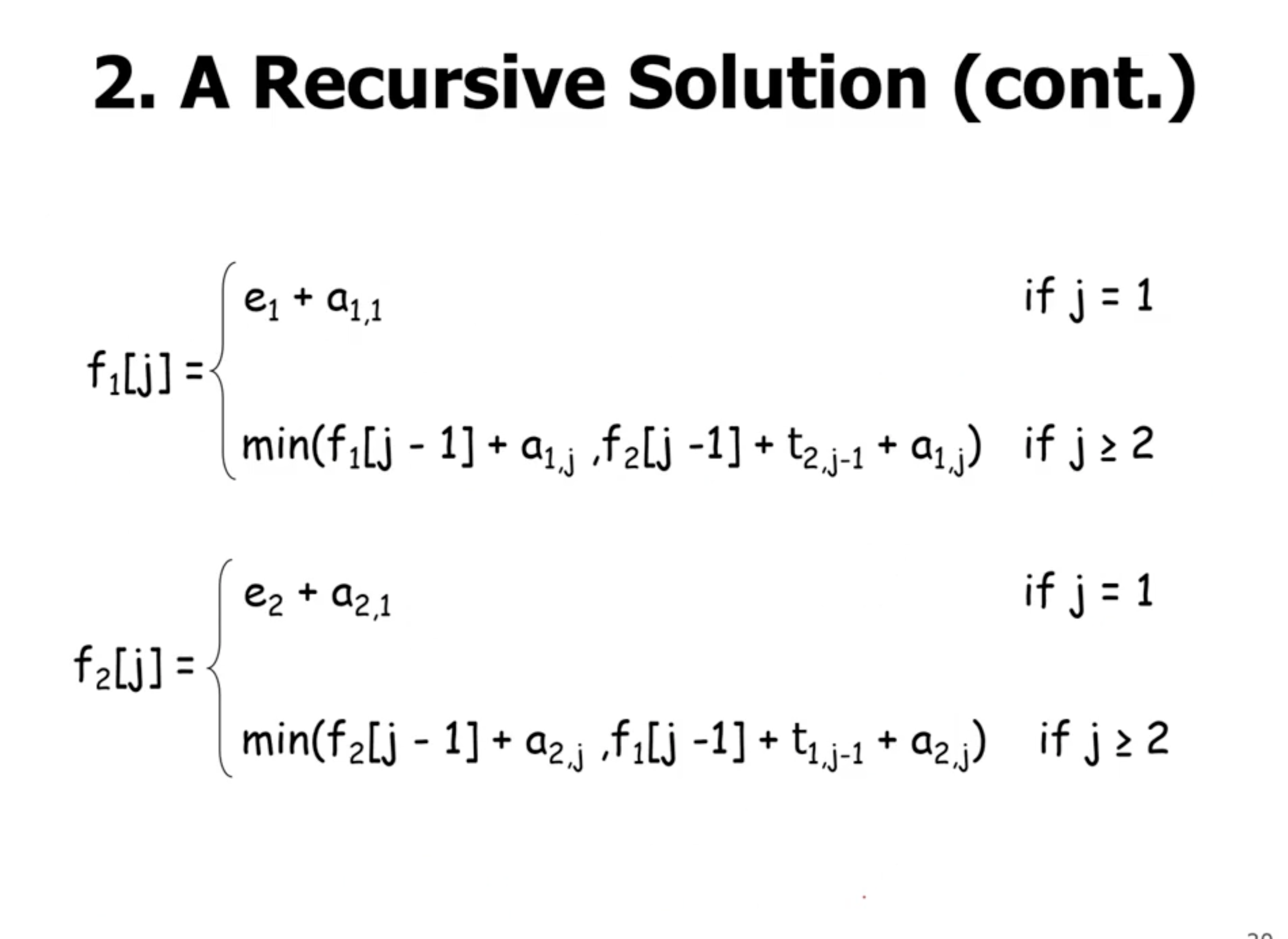
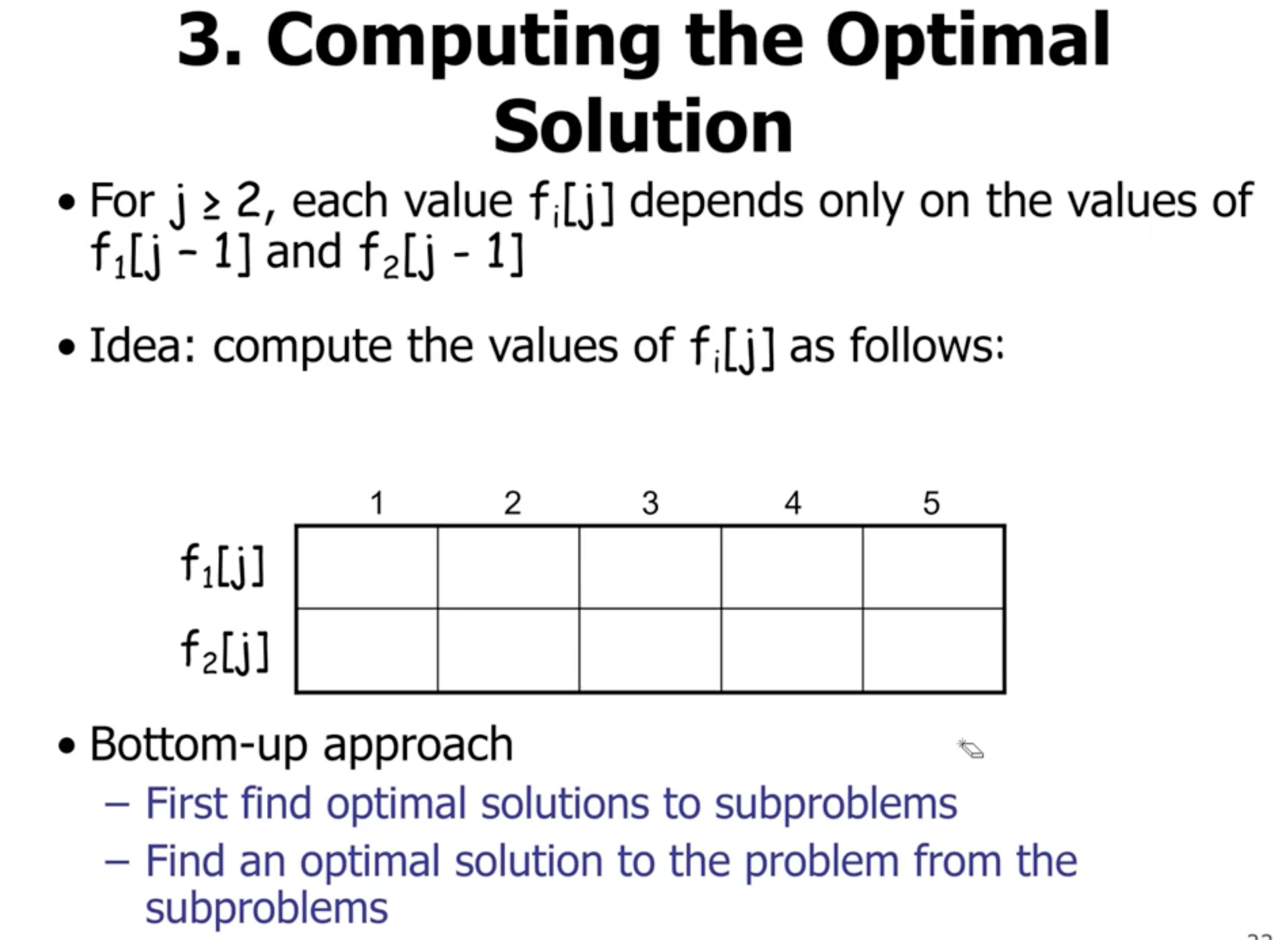
We want to solve this bottom up, which means we’ll start with the base cases.
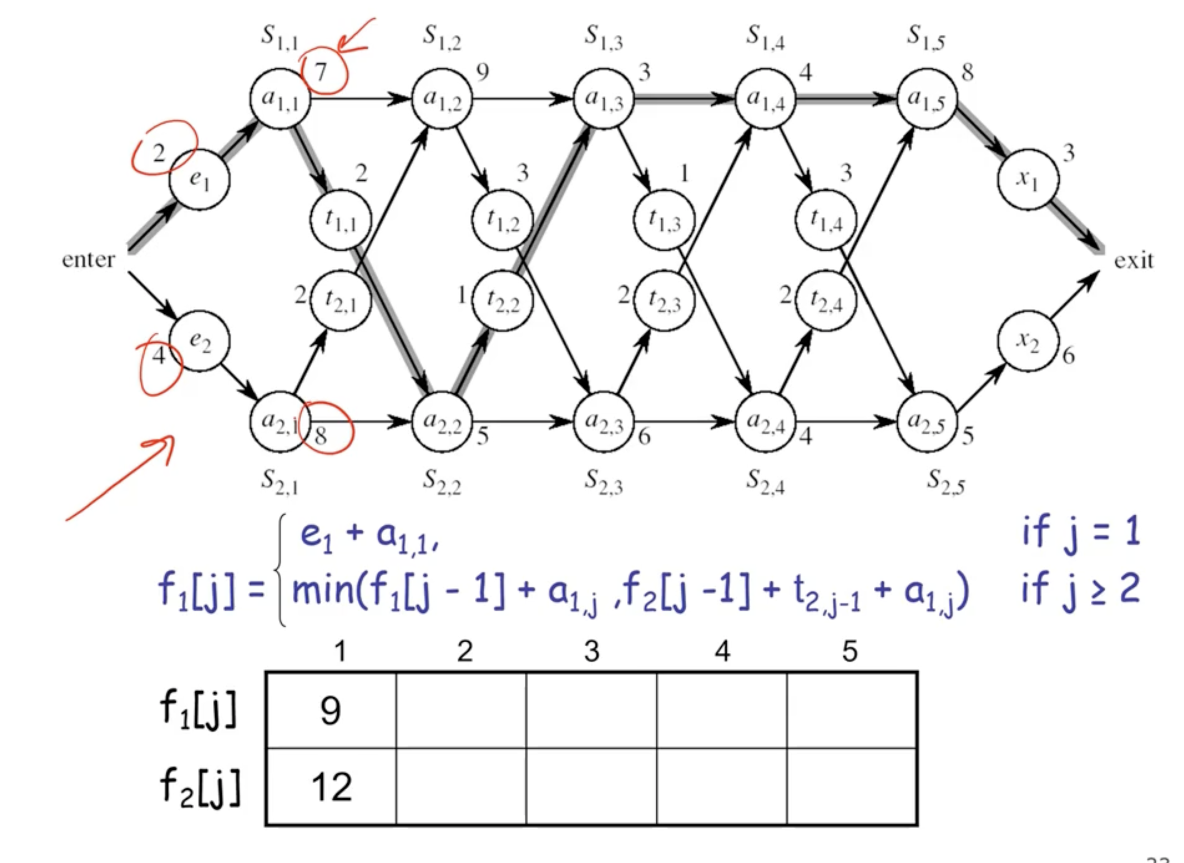
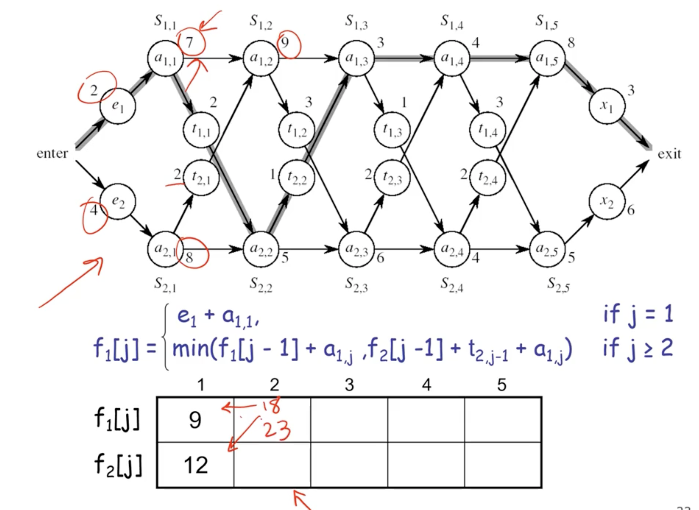
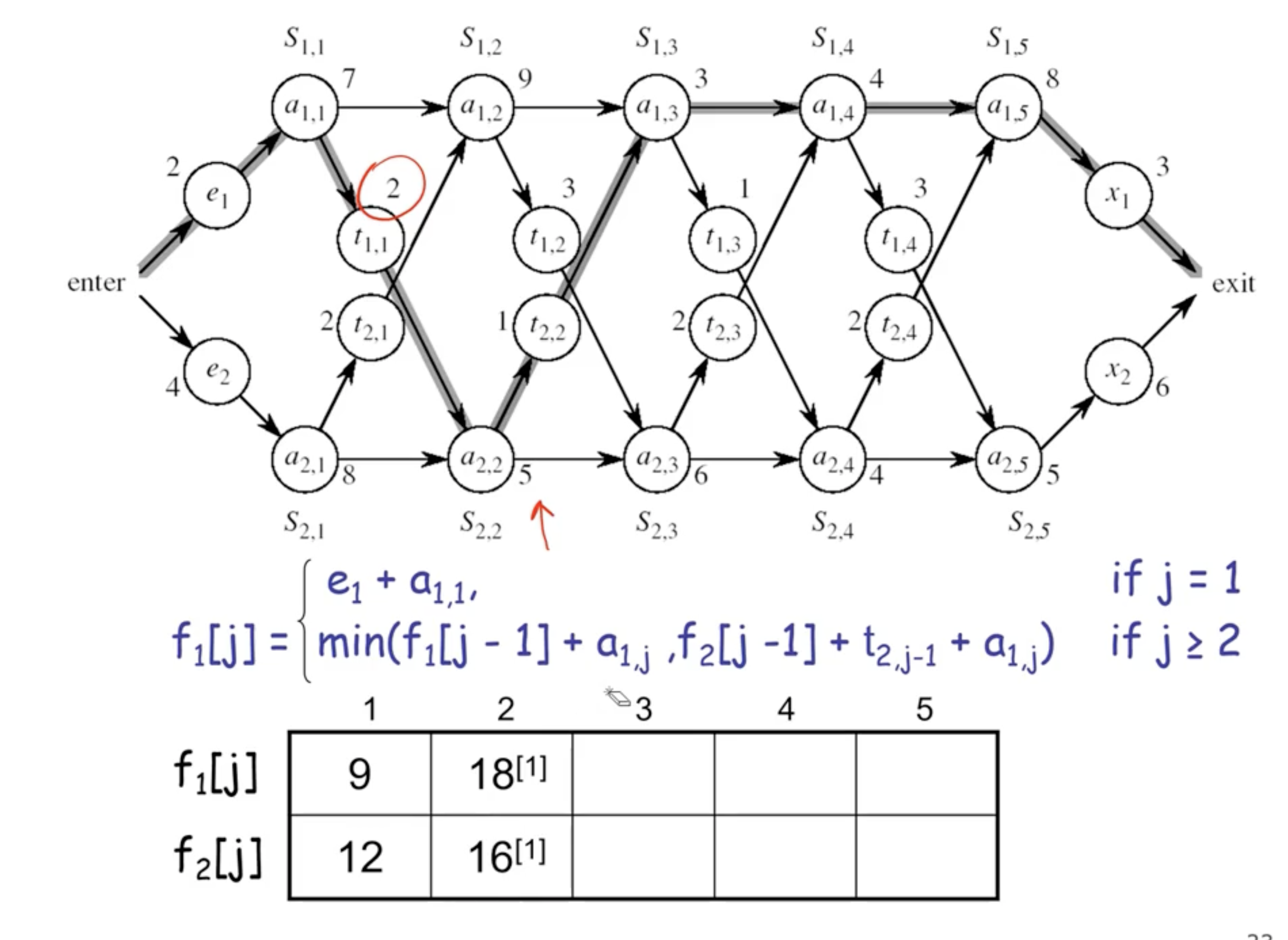
Note: \( 18^{[1]} \) indicates that the total time to exit the station is 18, coming from assembly 1.
- each cell is the solution to some sub problems
- you need an array big enough to fit the solution to each sub problem
- time complexity here is \( \Theta(n) \) .
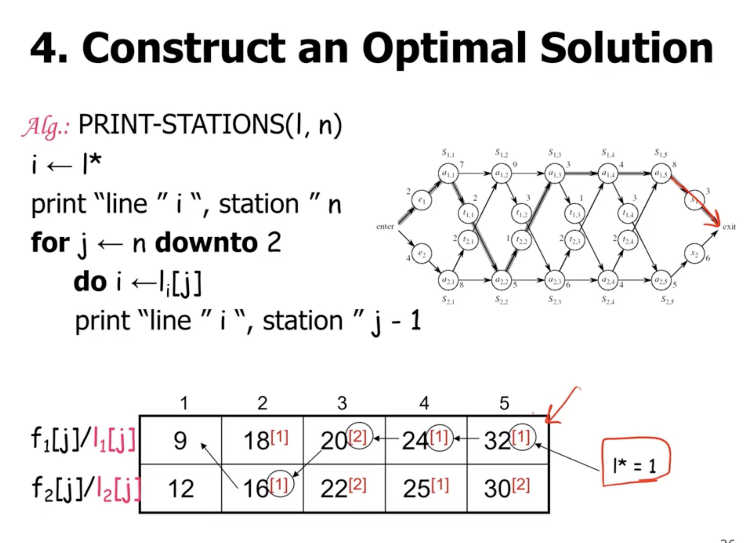
line 1 station 5
line 1 station 4
line 1 station 3
line 2 station 2
line 1 station 1